Reproducing Steve’s Code - Week 8

coding
week 8
renan
For Week 8 we are replicating Steve’s findings
Author
Affiliation

Master of Data Science Program @ The University of West Florida (UWF)

For the Week 8 we will continue to reproduce Steve’s findings with the dataset[1].

You can download the Dataset from the following link: Stroke Prediction Dataset

1. Setup and Data Loading

First we need to install all packages, system dependencies and solve conflicts to produce a new renv.lock file.

1.1 Load Libraries

Code
# Run this once to install all the necessary packages
# install.packages("dplyr")
# install.packages("car")
# install.packages("ResourceSelection")
# install.packages("caret")
# install.packages("rcompanion")
# install.packages("pROC")
# install.packages("cvAUC")

We can use this to check installed packages:

```{r}
renv::activate("website")
"yardstick" %in% rownames(installed.packages())
```
Code
# For data manipulation and visualization
library(tidyverse)
library(ggplot2)
library(corrplot)
library(knitr)
library(ggpubr)

# For data preprocessing and modeling
library(mice)
library(ROSE) # For SMOTE
library(ranger) # A fast implementation of random forests

# For stacking/ensemble models
library(stacks)
library(tidymodels)

library(themis)
library(gghighlight)

library(pscl)
library(dplyr)
library(car)
library(ResourceSelection)
library(caret)
library(rcompanion)
library(Hmisc)
library(pROC)
library(cvAUC)

# Set seed for reproducibility
set.seed(123)
ImportantPossible Dependencies Conflict

Need to further analyse if there are conflicts and System Dependency issues.

1.2 Load Data

Will be using my original Dataset as well Steve’s Dataset and compare for differences.

Renan: kaggle_data1 Steve: stroke1

1.2.1 Renan Dataset

Below will be loading the healthcare-dataset-stroke-data.csv and performing necessary changes to the dataset and loading into the DataFrame: kaggle_data1

Code
find_git_root <- function(start = getwd()) {
  path <- normalizePath(start, winslash = "/", mustWork = TRUE)
  while (path != dirname(path)) {
    if (dir.exists(file.path(path, ".git"))) return(path)
    path <- dirname(path)
  }
  stop("No .git directory found — are you inside a Git repository?")
}

repo_root <- find_git_root()
datasets_path <- file.path(repo_root, "datasets")
kaggle_dataset_path <- file.path(datasets_path, "kaggle-healthcare-dataset-stroke-data/healthcare-dataset-stroke-data.csv")
kaggle_data1 = read_csv(kaggle_dataset_path, show_col_types = FALSE)

# unique(kaggle_data1$bmi)
kaggle_data1 <- kaggle_data1 %>%
  mutate(bmi = na_if(bmi, "N/A")) %>%   # Convert "N/A" string to NA
  mutate(bmi = as.numeric(bmi))         # Convert from character to numeric

# Remove the 'Other' gender row and the 'id' column
kaggle_data1 <- kaggle_data1 %>%
  filter(gender != "Other") %>%
  select(-id) %>%
  mutate_if(is.character, as.factor) # Convert character columns to factors for easier modeling

1.2.1 Steve Dataset

Below will be loading the stroke.csv and performing necessary changes to the dataset and loading into the DataFrame: stroke1

Code
# Reading the datafile in (the same one you got for us Renan)#
steve_dataset_path <- file.path(datasets_path, "steve/stroke.csv")
stroke1 = read_csv(steve_dataset_path, show_col_types = FALSE)

1.3 Prepare Dataset

For each Column…removing the unncessary or unusable variables:

  1. Smoking Status - remove unknown
  2. bmi - remove N/A
  3. Work type - remove children
  4. age create numerical variable with 2 places after the decimal
  5. gender -remove other

Exploring Dataset so we can plan on how to proceed and possible changes.

Code
head(stroke1)
nrow(stroke1)
summary(stroke1)
count_tables <- lapply(stroke1, table)
count_tables

In each column..that has data points that are not usable, recoding those datapoints to become”N/A”

Code
stroke1[stroke1 == "N/A"] <- NA
stroke1[stroke1 == "Unknown"] <- NA
stroke1[stroke1 == "children"] <- NA
stroke1[stroke1 == "other"] <- NA

stroke1$bmi <- round(as.numeric(stroke1$bmi), 2)

stroke1$gender[stroke1$gender == "Male"] <- 1
stroke1$gender[stroke1$gender == "Female"] <- 2
stroke1$gender <- as.numeric(stroke1$gender)
Warning: NAs introduced by coercion
Code
stroke1$ever_married[stroke1$ever_married == "Yes"] <- 1
stroke1$ever_married[stroke1$ever_married == "No"] <- 2
stroke1$ever_married <- as.numeric(stroke1$ever_married)

stroke1$work_type[stroke1$work_type == "Govt_job"] <- 1
stroke1$work_type[stroke1$work_type == "Private"] <- 2
stroke1$work_type[stroke1$work_type == "Self-employed"] <- 3
stroke1$work_type[stroke1$work_type == "Never_worked"] <- 4
stroke1$work_type <- as.numeric(stroke1$work_type)

stroke1$Residence_type[stroke1$Residence_type == "Urban"] <- 1
stroke1$Residence_type[stroke1$Residence_type == "Rural"] <- 2
stroke1$Residence_type <- as.numeric(stroke1$Residence_type)

stroke1$avg_glucose_level <- as.numeric(stroke1$avg_glucose_level)

stroke1$heart_disease <- as.numeric(stroke1$heart_disease)

stroke1$hypertension <- as.numeric(stroke1$hypertension)

stroke1$age <- round(as.numeric(stroke1$age), 2)

stroke1$stroke <- as.numeric(stroke1$stroke)

stroke1$smoking_status[stroke1$smoking_status == "never smoked"] <- 1
stroke1$smoking_status[stroke1$smoking_status == "formerly smoked"] <- 2
stroke1$smoking_status[stroke1$smoking_status == "smokes"] <- 3
stroke1$smoking_status <- as.numeric(stroke1$smoking_status)

stroke1 <- stroke1[, !(names(stroke1) %in% "id")]
stroke1_clean <- na.omit(stroke1)

converted all columns to numeric and removed id

# converted all columns to numeric and removed id
str(stroke1_clean)
nrow(stroke1_clean)
LR_stroke1 <- stroke1_clean
str(LR_stroke1)
count_tables <- lapply(LR_stroke1, table)
count_tables

2. Apply Logistic Regression

Part 2:Create and Run the Logistic Regression model from the dataset

# Part 2:Create and Run the Logistic Regression model from the  dataset
model <- glm(stroke ~ gender + age + hypertension + heart_disease + ever_married + work_type + Residence_type + avg_glucose_level + bmi + smoking_status, data=LR_stroke1, family = binomial)
summary(model)

Call:
glm(formula = stroke ~ gender + age + hypertension + heart_disease + 
    ever_married + work_type + Residence_type + avg_glucose_level + 
    bmi + smoking_status, family = binomial, data = LR_stroke1)

Coefficients:
                   Estimate Std. Error z value Pr(>|z|)    
(Intercept)       -8.426854   0.873243  -9.650  < 2e-16 ***
gender             0.080370   0.167274   0.480 0.630893    
age                0.070967   0.006845  10.368  < 2e-16 ***
hypertension       0.570797   0.182580   3.126 0.001770 ** 
heart_disease      0.417884   0.220311   1.897 0.057856 .  
ever_married       0.174316   0.261832   0.666 0.505569    
work_type         -0.109615   0.126101  -0.869 0.384703    
Residence_type     0.005932   0.162188   0.037 0.970822    
avg_glucose_level  0.004658   0.001375   3.388 0.000704 ***
bmi                0.006275   0.012875   0.487 0.625954    
smoking_status     0.179921   0.106431   1.691 0.090932 .  
---
Signif. codes:  0 '***' 0.001 '**' 0.01 '*' 0.05 '.' 0.1 ' ' 1

(Dispersion parameter for binomial family taken to be 1)

    Null deviance: 1403.5  on 3356  degrees of freedom
Residual deviance: 1145.4  on 3346  degrees of freedom
AIC: 1167.4

Number of Fisher Scoring iterations: 7
ImportantIssue - Unbalanced Data set

The dataset is oversampling stroke rate by 77%.

Issue - Unbalanced Data set

The \(stroke rate = 180/3357 = 054%\) . But the stroke rate in the US is 3.1% by the CDC, AHA, and the NCHS.

The dataset is oversampling stroke rate by 77%. We can either SMOTE, under/over sample….but too much time

Best way is to recalibrate the intercept for this model (Ie change it here) so it can be used from now on

# Issue _ Unbalanced Data set #
# The stroke rate = 180/3357 = 054%. But the stroke rate in the US is 3.1% by the CDC, AHA, and the NCHS. #
# The dataset is oversampling stroke rate by 77%. We can either SMOTE, under/over sample....but too much time #
# Best way is to recalibrate the intercept for this model (Ie change it here) so it can be used from now on #
ds_prev <- .054
pop_prev <- .031
log_odds_ds <- qlogis(ds_prev)
log_odds_pop <- qlogis(pop_prev)
offset <- log_odds_pop - log_odds_ds
coefs <- coef(model)
coefs[1] <- coefs[1] + offset
print(coefs)
      (Intercept)            gender               age      hypertension 
     -9.005873116       0.080369937       0.070967479       0.570796782 
    heart_disease      ever_married         work_type    Residence_type 
      0.417883562       0.174315603      -0.109615162       0.005932360 
avg_glucose_level               bmi    smoking_status 
      0.004657820       0.006275415       0.179921439 

Original Intercept Coeff = -8.426854231

Changed intercept Coefficent to take into account current stroke rate or 3.1% = -9.005873116

all the other intercepts remain the same

3. Testing logistic Regression Model Assumptions

Part 3: Testing logistic Regression Model Assumptions

There are several assumptions for Logistic Regression. They are:

  1. The Dependent Variable is binary (i.e, 0 or 1)
  2. There is a linear relationship between th logit of the outcome and each predictor
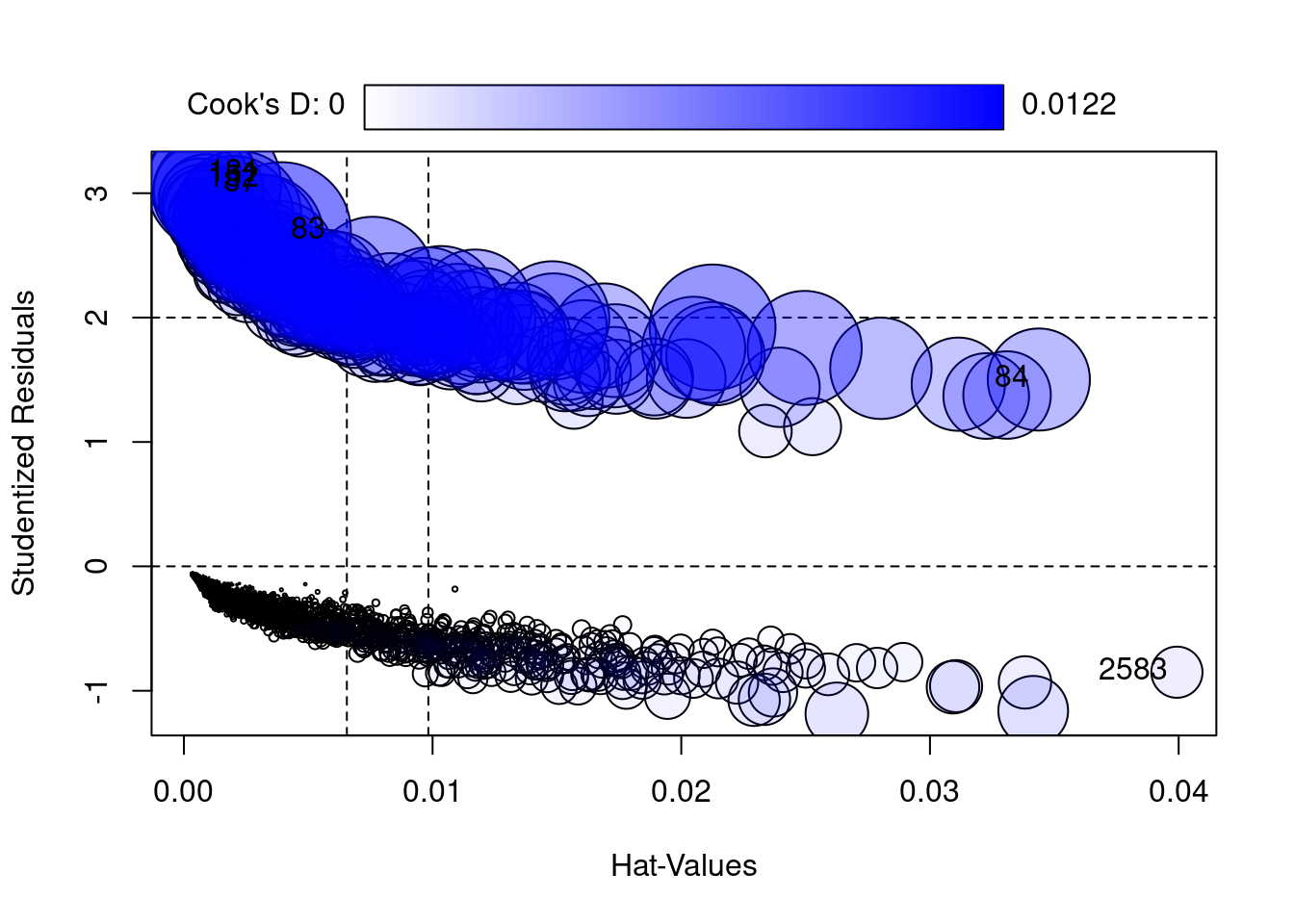
  3. There are NO high leverage outliers in the predictors
  4. There is No high multicollinearity (ie strong correlations) between predictors

3.1 Testing Assumption 1

Testing Assumption 1: The Dependent Variable is binary (0 or 1)

unique(LR_stroke1$stroke)
[1] 1 0

3.2 Testing Assumption 2

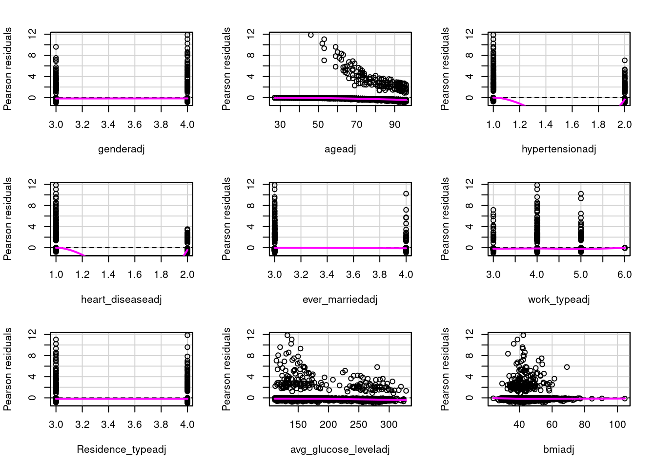
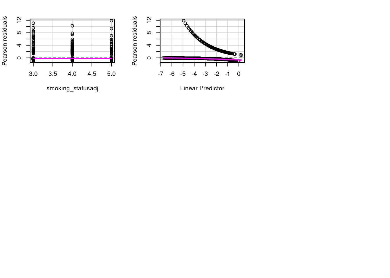
Testing Assumption 2: There is a linear relationship between the outcome variable and each predictor

first, adjust all predictors so all values are positive

Conclusion: For all continuous variables , ageadj, avg_glucose_leveladj, and bniadj, the residual plots show linearity

Conclusion: all the other predictors are categorical, with the magenta line flat, and the values clustering around certain values, they are also appropriate for logistic regression

Conclusion for assumption 2 - Linearity is met

LR_stroke1$genderadj <- LR_stroke1$gender + abs(min(LR_stroke1$gender)) + 1

LR_stroke1$ageadj <- LR_stroke1$age + abs(min(LR_stroke1$age)) + 1

LR_stroke1$hypertensionadj <- LR_stroke1$hypertension + abs(min(LR_stroke1$hypertension)) + 1

LR_stroke1$heart_diseaseadj <- LR_stroke1$heart_disease + abs(min(LR_stroke1$hypertension)) + 1

LR_stroke1$ever_marriedadj <- LR_stroke1$ever_married + abs(min(LR_stroke1$ever_married)) + 1

LR_stroke1$work_typeadj <- LR_stroke1$work_type + abs(min(LR_stroke1$work_type)) + 1

LR_stroke1$Residence_typeadj <- LR_stroke1$Residence_type + abs(min(LR_stroke1$Residence_type)) + 1

LR_stroke1$avg_glucose_leveladj <- LR_stroke1$avg_glucose_level + abs(min(LR_stroke1$avg_glucose_level)) + 1

LR_stroke1$bmiadj <- LR_stroke1$bmi + abs(min(LR_stroke1$bmi)) + 1

LR_stroke1$smoking_statusadj <- LR_stroke1$smoking_status + abs(min(LR_stroke1$smoking_status)) + 1

str(LR_stroke1)
tibble [3,357 × 21] (S3: tbl_df/tbl/data.frame)
 $ gender              : num [1:3357] 1 1 2 2 1 1 2 2 2 2 ...
 $ age                 : num [1:3357] 67 80 49 79 81 74 69 81 61 54 ...
 $ hypertension        : num [1:3357] 0 0 0 1 0 1 0 1 0 0 ...
 $ heart_disease       : num [1:3357] 1 1 0 0 0 1 0 0 1 0 ...
 $ ever_married        : num [1:3357] 1 1 1 1 1 1 2 1 1 1 ...
 $ work_type           : num [1:3357] 2 2 2 3 2 2 2 2 1 2 ...
 $ Residence_type      : num [1:3357] 1 2 1 2 1 2 1 2 2 1 ...
 $ avg_glucose_level   : num [1:3357] 229 106 171 174 186 ...
 $ bmi                 : num [1:3357] 36.6 32.5 34.4 24 29 27.4 22.8 29.7 36.8 27.3 ...
 $ smoking_status      : num [1:3357] 2 1 3 1 2 1 1 1 3 3 ...
 $ stroke              : num [1:3357] 1 1 1 1 1 1 1 1 1 1 ...
 $ genderadj           : num [1:3357] 3 3 4 4 3 3 4 4 4 4 ...
 $ ageadj              : num [1:3357] 81 94 63 93 95 88 83 95 75 68 ...
 $ hypertensionadj     : num [1:3357] 1 1 1 2 1 2 1 2 1 1 ...
 $ heart_diseaseadj    : num [1:3357] 2 2 1 1 1 2 1 1 2 1 ...
 $ ever_marriedadj     : num [1:3357] 3 3 3 3 3 3 4 3 3 3 ...
 $ work_typeadj        : num [1:3357] 4 4 4 5 4 4 4 4 3 4 ...
 $ Residence_typeadj   : num [1:3357] 3 4 3 4 3 4 3 4 4 3 ...
 $ avg_glucose_leveladj: num [1:3357] 285 162 227 230 242 ...
 $ bmiadj              : num [1:3357] 49.1 45 46.9 36.5 41.5 39.9 35.3 42.2 49.3 39.8 ...
 $ smoking_statusadj   : num [1:3357] 4 3 5 3 4 3 3 3 5 5 ...
 - attr(*, "na.action")= 'omit' Named int [1:1753] 2 9 10 14 20 24 28 30 32 39 ...
  ..- attr(*, "names")= chr [1:1753] "2" "9" "10" "14" ...
StrokeAdj <- LR_stroke1

StrokeAdj <- StrokeAdj[ , !(names(StrokeAdj) %in% c("gender", "age", "hypertension", "heart_disease", "ever_married", "work_type", "Residence_type", "avg_glucose_level", "bmi", "smoking_status")) ]

Fit the model

mod.2 <- glm(stroke ~ genderadj + ageadj + hypertensionadj + heart_diseaseadj + ever_marriedadj + work_typeadj + Residence_typeadj + avg_glucose_leveladj + bmiadj + smoking_statusadj, data=StrokeAdj, family=binomial)
# Plot Residuals
residualPlots(mod.2)

                     Test stat Pr(>|Test stat|)  
genderadj               0.0000          1.00000  
ageadj                  2.0626          0.15095  
hypertensionadj         0.0000          1.00000  
heart_diseaseadj        0.0000          1.00000  
ever_marriedadj         0.0000          1.00000  
work_typeadj            3.1406          0.07636 .
Residence_typeadj       0.0000          1.00000  
avg_glucose_leveladj    0.0103          0.91921  
bmiadj                  0.3947          0.52983  
smoking_statusadj       0.4775          0.48953  
---
Signif. codes:  0 '***' 0.001 '**' 0.01 '*' 0.05 '.' 0.1 ' ' 1

3.3 Testing Assumption 3

Testing Assumption 3: assess influential outliers using car package and influencePlot

alias(model)
Model :
stroke ~ gender + age + hypertension + heart_disease + ever_married + 
    work_type + Residence_type + avg_glucose_level + bmi + smoking_status
# install.packages("Hmisc")
# library(Hmisc)
rcorr(as.matrix(LR_stroke1))
                     gender   age hypertension heart_disease ever_married
gender                 1.00 -0.06        -0.04         -0.10         0.03
age                   -0.06  1.00         0.26          0.26        -0.49
hypertension          -0.04  0.26         1.00          0.11        -0.11
heart_disease         -0.10  0.26         0.11          1.00        -0.07
ever_married           0.03 -0.49        -0.11         -0.07         1.00
work_type              0.01  0.14         0.05          0.03        -0.02
Residence_type        -0.01 -0.02         0.00         -0.01         0.01
avg_glucose_level     -0.07  0.24         0.17          0.14        -0.12
bmi                   -0.02  0.04         0.13          0.00        -0.13
smoking_status        -0.08  0.03        -0.01          0.06        -0.06
stroke                -0.01  0.24         0.14          0.14        -0.07
genderadj              1.00 -0.06        -0.04         -0.10         0.03
ageadj                -0.06  1.00         0.26          0.26        -0.49
hypertensionadj       -0.04  0.26         1.00          0.11        -0.11
heart_diseaseadj      -0.10  0.26         0.11          1.00        -0.07
ever_marriedadj        0.03 -0.49        -0.11         -0.07         1.00
work_typeadj           0.01  0.14         0.05          0.03        -0.02
Residence_typeadj     -0.01 -0.02         0.00         -0.01         0.01
avg_glucose_leveladj  -0.07  0.24         0.17          0.14        -0.12
bmiadj                -0.02  0.04         0.13          0.00        -0.13
smoking_statusadj     -0.08  0.03        -0.01          0.06        -0.06
                     work_type Residence_type avg_glucose_level   bmi
gender                    0.01          -0.01             -0.07 -0.02
age                       0.14          -0.02              0.24  0.04
hypertension              0.05           0.00              0.17  0.13
heart_disease             0.03          -0.01              0.14  0.00
ever_married             -0.02           0.01             -0.12 -0.13
work_type                 1.00          -0.01              0.03 -0.02
Residence_type           -0.01           1.00              0.01  0.01
avg_glucose_level         0.03           0.01              1.00  0.16
bmi                      -0.02           0.01              0.16  1.00
smoking_status           -0.02          -0.04              0.01  0.03
stroke                    0.04          -0.01              0.14  0.01
genderadj                 0.01          -0.01             -0.07 -0.02
ageadj                    0.14          -0.02              0.24  0.04
hypertensionadj           0.05           0.00              0.17  0.13
heart_diseaseadj          0.03          -0.01              0.14  0.00
ever_marriedadj          -0.02           0.01             -0.12 -0.13
work_typeadj              1.00          -0.01              0.03 -0.02
Residence_typeadj        -0.01           1.00              0.01  0.01
avg_glucose_leveladj      0.03           0.01              1.00  0.16
bmiadj                   -0.02           0.01              0.16  1.00
smoking_statusadj        -0.02          -0.04              0.01  0.03
                     smoking_status stroke genderadj ageadj hypertensionadj
gender                        -0.08  -0.01      1.00  -0.06           -0.04
age                            0.03   0.24     -0.06   1.00            0.26
hypertension                  -0.01   0.14     -0.04   0.26            1.00
heart_disease                  0.06   0.14     -0.10   0.26            0.11
ever_married                  -0.06  -0.07      0.03  -0.49           -0.11
work_type                     -0.02   0.04      0.01   0.14            0.05
Residence_type                -0.04  -0.01     -0.01  -0.02            0.00
avg_glucose_level              0.01   0.14     -0.07   0.24            0.17
bmi                            0.03   0.01     -0.02   0.04            0.13
smoking_status                 1.00   0.02     -0.08   0.03           -0.01
stroke                         0.02   1.00     -0.01   0.24            0.14
genderadj                     -0.08  -0.01      1.00  -0.06           -0.04
ageadj                         0.03   0.24     -0.06   1.00            0.26
hypertensionadj               -0.01   0.14     -0.04   0.26            1.00
heart_diseaseadj               0.06   0.14     -0.10   0.26            0.11
ever_marriedadj               -0.06  -0.07      0.03  -0.49           -0.11
work_typeadj                  -0.02   0.04      0.01   0.14            0.05
Residence_typeadj             -0.04  -0.01     -0.01  -0.02            0.00
avg_glucose_leveladj           0.01   0.14     -0.07   0.24            0.17
bmiadj                         0.03   0.01     -0.02   0.04            0.13
smoking_statusadj              1.00   0.02     -0.08   0.03           -0.01
                     heart_diseaseadj ever_marriedadj work_typeadj
gender                          -0.10            0.03         0.01
age                              0.26           -0.49         0.14
hypertension                     0.11           -0.11         0.05
heart_disease                    1.00           -0.07         0.03
ever_married                    -0.07            1.00        -0.02
work_type                        0.03           -0.02         1.00
Residence_type                  -0.01            0.01        -0.01
avg_glucose_level                0.14           -0.12         0.03
bmi                              0.00           -0.13        -0.02
smoking_status                   0.06           -0.06        -0.02
stroke                           0.14           -0.07         0.04
genderadj                       -0.10            0.03         0.01
ageadj                           0.26           -0.49         0.14
hypertensionadj                  0.11           -0.11         0.05
heart_diseaseadj                 1.00           -0.07         0.03
ever_marriedadj                 -0.07            1.00        -0.02
work_typeadj                     0.03           -0.02         1.00
Residence_typeadj               -0.01            0.01        -0.01
avg_glucose_leveladj             0.14           -0.12         0.03
bmiadj                           0.00           -0.13        -0.02
smoking_statusadj                0.06           -0.06        -0.02
                     Residence_typeadj avg_glucose_leveladj bmiadj
gender                           -0.01                -0.07  -0.02
age                              -0.02                 0.24   0.04
hypertension                      0.00                 0.17   0.13
heart_disease                    -0.01                 0.14   0.00
ever_married                      0.01                -0.12  -0.13
work_type                        -0.01                 0.03  -0.02
Residence_type                    1.00                 0.01   0.01
avg_glucose_level                 0.01                 1.00   0.16
bmi                               0.01                 0.16   1.00
smoking_status                   -0.04                 0.01   0.03
stroke                           -0.01                 0.14   0.01
genderadj                        -0.01                -0.07  -0.02
ageadj                           -0.02                 0.24   0.04
hypertensionadj                   0.00                 0.17   0.13
heart_diseaseadj                 -0.01                 0.14   0.00
ever_marriedadj                   0.01                -0.12  -0.13
work_typeadj                     -0.01                 0.03  -0.02
Residence_typeadj                 1.00                 0.01   0.01
avg_glucose_leveladj              0.01                 1.00   0.16
bmiadj                            0.01                 0.16   1.00
smoking_statusadj                -0.04                 0.01   0.03
                     smoking_statusadj
gender                           -0.08
age                               0.03
hypertension                     -0.01
heart_disease                     0.06
ever_married                     -0.06
work_type                        -0.02
Residence_type                   -0.04
avg_glucose_level                 0.01
bmi                               0.03
smoking_status                    1.00
stroke                            0.02
genderadj                        -0.08
ageadj                            0.03
hypertensionadj                  -0.01
heart_diseaseadj                  0.06
ever_marriedadj                  -0.06
work_typeadj                     -0.02
Residence_typeadj                -0.04
avg_glucose_leveladj              0.01
bmiadj                            0.03
smoking_statusadj                 1.00

n= 3357 


P
                     gender age    hypertension heart_disease ever_married
gender                      0.0012 0.0204       0.0000        0.1140      
age                  0.0012        0.0000       0.0000        0.0000      
hypertension         0.0204 0.0000              0.0000        0.0000      
heart_disease        0.0000 0.0000 0.0000                     0.0000      
ever_married         0.1140 0.0000 0.0000       0.0000                    
work_type            0.3863 0.0000 0.0051       0.0862        0.2313      
Residence_type       0.5077 0.3076 0.8569       0.5527        0.5150      
avg_glucose_level    0.0000 0.0000 0.0000       0.0000        0.0000      
bmi                  0.2487 0.0144 0.0000       0.8185        0.0000      
smoking_status       0.0000 0.0448 0.7537       0.0005        0.0009      
stroke               0.4296 0.0000 0.0000       0.0000        0.0002      
genderadj            0.0000 0.0012 0.0204       0.0000        0.1140      
ageadj               0.0012 0.0000 0.0000       0.0000        0.0000      
hypertensionadj      0.0204 0.0000 0.0000       0.0000        0.0000      
heart_diseaseadj     0.0000 0.0000 0.0000       0.0000        0.0000      
ever_marriedadj      0.1140 0.0000 0.0000       0.0000        0.0000      
work_typeadj         0.3863 0.0000 0.0051       0.0862        0.2313      
Residence_typeadj    0.5077 0.3076 0.8569       0.5527        0.5150      
avg_glucose_leveladj 0.0000 0.0000 0.0000       0.0000        0.0000      
bmiadj               0.2487 0.0144 0.0000       0.8185        0.0000      
smoking_statusadj    0.0000 0.0448 0.7537       0.0005        0.0009      
                     work_type Residence_type avg_glucose_level bmi   
gender               0.3863    0.5077         0.0000            0.2487
age                  0.0000    0.3076         0.0000            0.0144
hypertension         0.0051    0.8569         0.0000            0.0000
heart_disease        0.0862    0.5527         0.0000            0.8185
ever_married         0.2313    0.5150         0.0000            0.0000
work_type                      0.6768         0.0467            0.3243
Residence_type       0.6768                   0.6427            0.5689
avg_glucose_level    0.0467    0.6427                           0.0000
bmi                  0.3243    0.5689         0.0000                  
smoking_status       0.3764    0.0208         0.7679            0.0925
stroke               0.0259    0.7171         0.0000            0.6866
genderadj            0.3863    0.5077         0.0000            0.2487
ageadj               0.0000    0.3076         0.0000            0.0144
hypertensionadj      0.0051    0.8569         0.0000            0.0000
heart_diseaseadj     0.0862    0.5527         0.0000            0.8185
ever_marriedadj      0.2313    0.5150         0.0000            0.0000
work_typeadj         0.0000    0.6768         0.0467            0.3243
Residence_typeadj    0.6768    0.0000         0.6427            0.5689
avg_glucose_leveladj 0.0467    0.6427         0.0000            0.0000
bmiadj               0.3243    0.5689         0.0000            0.0000
smoking_statusadj    0.3764    0.0208         0.7679            0.0925
                     smoking_status stroke genderadj ageadj hypertensionadj
gender               0.0000         0.4296 0.0000    0.0012 0.0204         
age                  0.0448         0.0000 0.0012    0.0000 0.0000         
hypertension         0.7537         0.0000 0.0204    0.0000 0.0000         
heart_disease        0.0005         0.0000 0.0000    0.0000 0.0000         
ever_married         0.0009         0.0002 0.1140    0.0000 0.0000         
work_type            0.3764         0.0259 0.3863    0.0000 0.0051         
Residence_type       0.0208         0.7171 0.5077    0.3076 0.8569         
avg_glucose_level    0.7679         0.0000 0.0000    0.0000 0.0000         
bmi                  0.0925         0.6866 0.2487    0.0144 0.0000         
smoking_status                      0.2559 0.0000    0.0448 0.7537         
stroke               0.2559                0.4296    0.0000 0.0000         
genderadj            0.0000         0.4296           0.0012 0.0204         
ageadj               0.0448         0.0000 0.0012           0.0000         
hypertensionadj      0.7537         0.0000 0.0204    0.0000                
heart_diseaseadj     0.0005         0.0000 0.0000    0.0000 0.0000         
ever_marriedadj      0.0009         0.0002 0.1140    0.0000 0.0000         
work_typeadj         0.3764         0.0259 0.3863    0.0000 0.0051         
Residence_typeadj    0.0208         0.7171 0.5077    0.3076 0.8569         
avg_glucose_leveladj 0.7679         0.0000 0.0000    0.0000 0.0000         
bmiadj               0.0925         0.6866 0.2487    0.0144 0.0000         
smoking_statusadj    0.0000         0.2559 0.0000    0.0448 0.7537         
                     heart_diseaseadj ever_marriedadj work_typeadj
gender               0.0000           0.1140          0.3863      
age                  0.0000           0.0000          0.0000      
hypertension         0.0000           0.0000          0.0051      
heart_disease        0.0000           0.0000          0.0862      
ever_married         0.0000           0.0000          0.2313      
work_type            0.0862           0.2313          0.0000      
Residence_type       0.5527           0.5150          0.6768      
avg_glucose_level    0.0000           0.0000          0.0467      
bmi                  0.8185           0.0000          0.3243      
smoking_status       0.0005           0.0009          0.3764      
stroke               0.0000           0.0002          0.0259      
genderadj            0.0000           0.1140          0.3863      
ageadj               0.0000           0.0000          0.0000      
hypertensionadj      0.0000           0.0000          0.0051      
heart_diseaseadj                      0.0000          0.0862      
ever_marriedadj      0.0000                           0.2313      
work_typeadj         0.0862           0.2313                      
Residence_typeadj    0.5527           0.5150          0.6768      
avg_glucose_leveladj 0.0000           0.0000          0.0467      
bmiadj               0.8185           0.0000          0.3243      
smoking_statusadj    0.0005           0.0009          0.3764      
                     Residence_typeadj avg_glucose_leveladj bmiadj
gender               0.5077            0.0000               0.2487
age                  0.3076            0.0000               0.0144
hypertension         0.8569            0.0000               0.0000
heart_disease        0.5527            0.0000               0.8185
ever_married         0.5150            0.0000               0.0000
work_type            0.6768            0.0467               0.3243
Residence_type       0.0000            0.6427               0.5689
avg_glucose_level    0.6427            0.0000               0.0000
bmi                  0.5689            0.0000               0.0000
smoking_status       0.0208            0.7679               0.0925
stroke               0.7171            0.0000               0.6866
genderadj            0.5077            0.0000               0.2487
ageadj               0.3076            0.0000               0.0144
hypertensionadj      0.8569            0.0000               0.0000
heart_diseaseadj     0.5527            0.0000               0.8185
ever_marriedadj      0.5150            0.0000               0.0000
work_typeadj         0.6768            0.0467               0.3243
Residence_typeadj                      0.6427               0.5689
avg_glucose_leveladj 0.6427                                 0.0000
bmiadj               0.5689            0.0000                     
smoking_statusadj    0.0208            0.7679               0.0925
                     smoking_statusadj
gender               0.0000           
age                  0.0448           
hypertension         0.7537           
heart_disease        0.0005           
ever_married         0.0009           
work_type            0.3764           
Residence_type       0.0208           
avg_glucose_level    0.7679           
bmi                  0.0925           
smoking_status       0.0000           
stroke               0.2559           
genderadj            0.0000           
ageadj               0.0448           
hypertensionadj      0.7537           
heart_diseaseadj     0.0005           
ever_marriedadj      0.0009           
work_typeadj         0.3764           
Residence_typeadj    0.0208           
avg_glucose_leveladj 0.7679           
bmiadj               0.0925           
smoking_statusadj                     
# install.packages("car")
# library(car)
influencePlot(model)

        StudRes          Hat       CookD
83    2.6917353 0.0039267816 0.012237368
84    1.5018344 0.0343771041 0.006641860
87    3.0732709 0.0012042796 0.011476828
131   3.1608870 0.0006013465 0.007697762
152   3.1135601 0.0005613972 0.006237531
2583 -0.8509399 0.0399302730 0.001668526

Cooks D ranges from 0 to .0122

While the ideal size is 4/N (4/3357 = 0.012), its far outside the danger zone of .5

Conclusion: Assumption 3 is met - No substantial outliers

3.4 Testing Assumption 4

Testing Assumption 4 : Multicollinearity using vif in the care package

vif(model)
           gender               age      hypertension     heart_disease 
         1.041499          1.213552          1.051213          1.083661 
     ever_married         work_type    Residence_type avg_glucose_level 
         1.018892          1.051698          1.006965          1.105268 
              bmi    smoking_status 
         1.117138          1.049260 

Conclusion. All vif values are below 5 or 10. Ideally most values should be around 1. Range for all

the predictors is between: 1.01 - 1.21. Way below the danger threshold of 5 to 10.

Conclusion: No Multicollinearity

Final Conclusion: All4 assumptions are met, logistic regression is a valid model

3.5 Conclusion of Testing Assumptions

Final Conclusion: All 4 assumptions are met, logistic regression is a valid model

4 Analysis of the Model

Part 4: Analysis of the Model

There are 2 issues with the model. Fit and Predictive Capability

4.1 Use Hosmer-lemesho and Naglekerke R

Part 1 fit. Use Hosmer-lemesho and Naglekerke R for non technical audience

# install.packages("ResourceSelection")
# library(ResourceSelection)
hoslem.test(model$y, fitted(model), g = 10)

    Hosmer and Lemeshow goodness of fit (GOF) test

data:  model$y, fitted(model)
X-squared = 5.2704, df = 8, p-value = 0.7283
# install.packages("rcompanion")
# library(rcompanion)
nagelkerke(model)
$Models
                                                                                                                                                                               
Model: "glm, stroke ~ gender + age + hypertension + heart_disease + ever_married + work_type + Residence_type + avg_glucose_level + bmi + smoking_status, binomial, LR_stroke1"
Null:  "glm, stroke ~ 1, binomial, LR_stroke1"                                                                                                                                 

$Pseudo.R.squared.for.model.vs.null
                             Pseudo.R.squared
McFadden                            0.1838790
Cox and Snell (ML)                  0.0739944
Nagelkerke (Cragg and Uhler)        0.2165560

$Likelihood.ratio.test
 Df.diff LogLik.diff  Chisq    p.value
     -10     -129.03 258.07 1.0892e-49

$Number.of.observations
           
Model: 3357
Null:  3357

$Messages
[1] "Note: For models fit with REML, these statistics are based on refitting with ML"

$Warnings
[1] "None"

4.2 Predictive Capability

Part 2 - Predictive Capability

# install.packages("pROC")
# library(pROC)
probs <- predict(model, type = "response")
roc_obj <- roc(LR_stroke1$stroke, probs)
Setting levels: control = 0, case = 1
Setting direction: controls < cases
auc(roc_obj)
Area under the curve: 0.8285

Predict AUC cross validation

NoteNeed to implement AUC cross validation

Could not understand yet how to implement the AUC cross validation

# Predict AUC cross validation
# install.packages("cvAUC")
# library(cvAUC)

Confusion Matrix

# Confusion Matrix
LR_stroke1$gender <- factor(LR_stroke1$gender)
LR_stroke1$hypertension <- factor(LR_stroke1$hypertension)
LR_stroke1$heart_disease <- factor(LR_stroke1$heart_disease)
LR_stroke1$ever_married <- factor(LR_stroke1$ever_married)
LR_stroke1$work_type <- factor(LR_stroke1$work_type)
LR_stroke1$Residence_type <- factor(LR_stroke1$Residence_type)
LR_stroke1$smoking_status <- factor(LR_stroke1$smoking_status)
LR_stroke1$stroke <- factor(LR_stroke1$stroke)

fit logistic regression model

# fit logistic regression model
model_CM <- glm(stroke ~ gender + age + hypertension + heart_disease + ever_married + work_type + Residence_type + avg_glucose_level + bmi + smoking_status, data=LR_stroke1, family = binomial)

Get Predicted Probabilities for each observation

# Get Predicted Probabilities for each observation
pred_prob <- predict(model_CM, type = "response")

create 10 confusion matrices at threshold intervals between 1 and 0 to create a ROC

Classify prediction using a threshold (0.5 is common but can adjust)

IF 1 row is all 0’s then model doesn’t show any predictability

At threshold of around 1.0

# create 10 confusion matrices at threshold intervals between 1 and 0 to create a ROC
# Classify prediction using a threshold (0.5 is common but can adjust)
# IF 1 row is all 0's then model doesn't show any predictability
# At threshold of around 1.0
pred_class <- factor(ifelse(pred_prob > .99, 1, 0), levels = c(0, 1))
conf_matrix <- confusionMatrix(pred_class, factor(LR_stroke1$stroke, levels = c("0", "1")), positive = "1")
print(conf_matrix$table)
          Reference
Prediction    0    1
         0 3177  180
         1    0    0

IF 1 row is all 0’s then model doesn’t show any predictability

At threshold of 0.9

# At threshold of 0.9
pred_class <- factor(ifelse(pred_prob > 0.9, 1, 0), levels = c(0, 1))
conf_matrix <- confusionMatrix(pred_class, factor(LR_stroke1$stroke, levels = c("0", "1")), positive = "1")
print(conf_matrix$table)
          Reference
Prediction    0    1
         0 3177  180
         1    0    0

IF 1 row is all 0’s then model doesn’t show any predictability

At threshold of 0.8

# At threshold of 0.8
pred_class <- factor(ifelse(pred_prob > 0.8, 1, 0), levels = c(0, 1))
conf_matrix <- confusionMatrix(pred_class, factor(LR_stroke1$stroke, levels = c("0", "1")), positive = "1")
print(conf_matrix$table)
          Reference
Prediction    0    1
         0 3177  180
         1    0    0

IF 1 row is all 0’s then model doesn’t show any predictability

At threshold of 0.7

# At threshold of 0.7
pred_class <- factor(ifelse(pred_prob > 0.7, 1, 0), levels = c(0, 1))
conf_matrix <- confusionMatrix(pred_class, factor(LR_stroke1$stroke, levels = c("0", "1")), positive = "1")
print(conf_matrix$table)
          Reference
Prediction    0    1
         0 3177  180
         1    0    0

At threshold of 0.6

# At threshold of 0.6
pred_class <- factor(ifelse(pred_prob > 0.6, 1, 0), levels = c(0, 1))
conf_matrix <- confusionMatrix(pred_class, factor(LR_stroke1$stroke, levels = c("0", "1")), positive = "1")
print(conf_matrix$table)
          Reference
Prediction    0    1
         0 3177  179
         1    0    1

at threshold of 0.6 that starts the models predictability

Extract precision,Recall and F1 from confusion matrix using the caret package

# Extract precision, Recall and F1 from confusion matrix using the caret package
precision <- conf_matrix$byClass["Pos Pred Value"] 
recall <- conf_matrix$byClass["Sensitivity"]
f1 <- 2 * ((precision * recall)/ (precision + recall))
print(sprintf("F1: %f", f1))
[1] "F1: 0.011050"
print(sprintf("recall: %f", recall))
[1] "recall: 0.005556"
print(sprintf("precision: %f", precision))
[1] "precision: 1.000000"

at threshold of 0.5

# at threshold of 0.5
pred_class <- factor(ifelse(pred_prob > 0.5, 1, 0), levels = c(0, 1))
conf_matrix <- confusionMatrix(pred_class, factor(LR_stroke1$stroke, levels = c("0", "1")), positive = "1")
print(conf_matrix$table)
          Reference
Prediction    0    1
         0 3176  179
         1    1    1

Extract precision,Recall and F1 from confusion matrix using the caret package

# Extract precision,Recall and F1 from confusion matrix using the caret package
precision <- conf_matrix$byClass["Pos Pred Value"] 
recall <- conf_matrix$byClass["Sensitivity"]
f1 <- 2 * ((precision * recall)/ (precision + recall))
print(sprintf("F1: %f", f1))
[1] "F1: 0.010989"
print(sprintf("recall: %f", recall))
[1] "recall: 0.005556"
print(sprintf("precision: %f", precision))
[1] "precision: 0.500000"

At threshold of 0.4

# At threshold of 0.4
pred_class <- factor(ifelse(pred_prob > 0.4, 1, 0), levels = c(0, 1))
conf_matrix <- confusionMatrix(pred_class, factor(LR_stroke1$stroke, levels = c("0", "1")), positive = "1")
print(conf_matrix$table)
          Reference
Prediction    0    1
         0 3171  174
         1    6    6

Extract precision,Recall and F1 from confusion matrix using the caret package

# Extract precision,Recall and F1 from confusion matrix using the caret package
precision <- conf_matrix$byClass["Pos Pred Value"] 
recall <- conf_matrix$byClass["Sensitivity"]
f1 <- 2 * ((precision * recall)/ (precision + recall))
print(sprintf("F1: %f", f1))
[1] "F1: 0.062500"
print(sprintf("recall: %f", recall))
[1] "recall: 0.033333"
print(sprintf("precision: %f", precision))
[1] "precision: 0.500000"

at threshold of 0.3

# at threshold of 0.3
pred_class <- factor(ifelse(pred_prob > 0.3, 1, 0), levels = c(0, 1))
conf_matrix <- confusionMatrix(pred_class, factor(LR_stroke1$stroke, levels = c("0", "1")), positive = "1")
print(conf_matrix$table)
          Reference
Prediction    0    1
         0 3140  164
         1   37   16

Extract precision,Recall and F1 from confusion matrix using the caret package

# Extract precision,Recall and F1 from confusion matrix using the caret package
precision <- conf_matrix$byClass["Pos Pred Value"] 
recall <- conf_matrix$byClass["Sensitivity"]
f1 <- 2 * ((precision * recall)/ (precision + recall))
print(sprintf("F1: %f", f1))
[1] "F1: 0.137339"
print(sprintf("recall: %f", recall))
[1] "recall: 0.088889"
print(sprintf("precision: %f", precision))
[1] "precision: 0.301887"

at threshold of 0.2

# at threshold of 0.2
pred_class <- factor(ifelse(pred_prob > 0.2, 1, 0), levels = c(0, 1))
conf_matrix <- confusionMatrix(pred_class, factor(LR_stroke1$stroke, levels = c("0", "1")), positive = "1")
print(conf_matrix$table)
          Reference
Prediction    0    1
         0 3040  134
         1  137   46

Extract precision,Recall and F1 from confusion matrix using the caret package

# Extract precision,Recall and F1 from confusion matrix using the caret package
precision <- conf_matrix$byClass["Pos Pred Value"] 
recall <- conf_matrix$byClass["Sensitivity"]
f1 <- 2 * ((precision * recall)/ (precision + recall))
print(sprintf("F1: %f", f1))
[1] "F1: 0.253444"
print(sprintf("recall: %f", recall))
[1] "recall: 0.255556"
print(sprintf("precision: %f", precision))
[1] "precision: 0.251366"

Using the different Confusion Matrices, Create the ROC curve

Conclusion

The code is unreadable and has several mistakes from Syntax to several implementation errors and System dependencies that I could not meet. So I had to do my best interpretation to reproduce it in Quarto.

  • Ideas for improving precision, recall and f1_score
  • Address imbalance by upsample (add stroke cases), downsample (remove non strokecases) and or SMOTE (Synthetic data)
  • Change the classification threshold
  • Compare with Alternative Models such as random forrests or XGBoost

References

1. fedesoriano. (n.d.). Stroke Prediction Dataset. https://www.kaggle.com/datasets/fedesoriano/stroke-prediction-dataset