Reproducing Steve’s Code - Week 7

coding

week 7

renan

For Week 7 we are replicating Steve’s findings

Author

Affiliation

Renan Monteiro Barbosa

Master of Data Science Program @ The University of West Florida (UWF)

For the Week 7 we will be reproducing Steve’s findings with the dataset^[1].

You can download the Dataset from the following link: Stroke Prediction Dataset

1. Setup and Data Loading

First we need to install all packages, system dependencies and solve conflicts to produce a new renv.lock file.

1.1 Load Libraries

Code

# Run this once to install all the necessary packages
# install.packages(c("corrplot", "ggpubr", "caret", "mice", "ROSE", "ranger", "stacks", "tidymodels"))
# install.packages("themis")
# install.packages("xgboost")
# install.packages("gghighlight")
# install.packages("dplyr")
# install.packages("pscl")
# install.packages("parallelly")
# install.packages("cli")
# install.packages("car")
# install.packages("ResourceSelection")

We can use this to check installed packages:

```{r}
renv::activate("website")
"yardstick" %in% rownames(installed.packages())
```

Code

# For data manipulation and visualization
library(tidyverse)
library(ggplot2)
library(corrplot)
library(knitr)
library(ggpubr)

# For data preprocessing and modeling
library(caret)
library(mice)
library(ROSE) # For SMOTE
library(ranger) # A fast implementation of random forests

# For stacking/ensemble models
library(stacks)
library(tidymodels)

library(themis)
library(gghighlight)

library(dplyr)
library(pscl)
library(car)
library(ResourceSelection)

# Set seed for reproducibility
set.seed(123)

1.2 Load Data

Will be using my original Dataset as well Steve’s Dataset and compare for differences.

Renan: kaggle_data1 Steve: stroke1

1.2.1 Renan Dataset

Below will be loading the healthcare-dataset-stroke-data.csv and performing necessary changes to the dataset and loading into the DataFrame: kaggle_data1

Code

find_git_root <- function(start = getwd()) {
  path <- normalizePath(start, winslash = "/", mustWork = TRUE)
  while (path != dirname(path)) {
    if (dir.exists(file.path(path, ".git"))) return(path)
    path <- dirname(path)
  }
  stop("No .git directory found — are you inside a Git repository?")
}

repo_root <- find_git_root()
datasets_path <- file.path(repo_root, "datasets")
kaggle_dataset_path <- file.path(datasets_path, "kaggle-healthcare-dataset-stroke-data/healthcare-dataset-stroke-data.csv")
kaggle_data1 = read_csv(kaggle_dataset_path, show_col_types = FALSE)

# unique(kaggle_data1$bmi)
kaggle_data1 <- kaggle_data1 %>%
  mutate(bmi = na_if(bmi, "N/A")) %>%   # Convert "N/A" string to NA
  mutate(bmi = as.numeric(bmi))         # Convert from character to numeric

# Remove the 'Other' gender row and the 'id' column
kaggle_data1 <- kaggle_data1 %>%
  filter(gender != "Other") %>%
  select(-id) %>%
  mutate_if(is.character, as.factor) # Convert character columns to factors for easier modeling

1.2.1 Steve Dataset

Below will be loading the stroke.csv and performing necessary changes to the dataset and loading into the DataFrame: stroke1

Code

# Reading the datafile in (the same one you got for us Renan)#
steve_dataset_path <- file.path(datasets_path, "steve/stroke.csv")
stroke1 = read_csv(steve_dataset_path, show_col_types = FALSE)
# stroke1 <- read.csv("D:\\stroke.csv")

Exploring Dataset so we can plan on how to proceed and possible changes.

Code

# Reveiewing the columns of the data and the dataset size#
head(stroke1)
nrow(stroke1)
#Some data to look at the data in each column#
summary(stroke1)
count_tables <- lapply(stroke1, table)
count_tables

Preparing the Dataset

For each Column…removing the unncessary or unusable variables: 1. Smoking Status - remove unknown 1. bmi - remove N/A 3. Work type - remove children 4. age create numerical variable with 2 places after the decimal 5. gender -remove other

In each column..that has data points that are not usable, recoding those datapoints to become”N/A”

Code

stroke1[stroke1 == "N/A"] <- NA
stroke1[stroke1 == "Unknown"] <- NA
stroke1[stroke1 == "children"] <- NA
stroke1[stroke1 == "other"] <- NA

for BMI changing the variable type to numeric and formatting the data point to 2 places ater the decimal

Code

stroke1$bmi <- round(as.numeric(stroke1$bmi), 2)

For Gender, changning Male to 1 and Female to 2, then reformatting gender as numeric

Code

stroke1$gender[stroke1$gender == "Male"] <- 1
stroke1$gender[stroke1$gender == "Female"] <- 2
stroke1$gender <- as.numeric(stroke1$gender)

Warning: NAs introduced by coercion

For ever_married, changing yes to 1 and No to 2, the reformatting the variable ever_married to numeric

Code

stroke1$ever_married[stroke1$ever_married == "Yes"] <- 1
stroke1$ever_married[stroke1$ever_married == "No"] <- 2
stroke1$ever_married <- as.numeric(stroke1$ever_married)

For work type recoding Govt_job to 1, Private to 3, Self-employed to 3, and Never_worked to 4, then reformatting work_type to numeric

Code

stroke1$work_type[stroke1$work_type == "Govt_job"] <- 1
stroke1$work_type[stroke1$work_type == "Private"] <- 2
stroke1$work_type[stroke1$work_type == "Self-employed"] <- 3
stroke1$work_type[stroke1$work_type == "Never_worked"] <- 4
stroke1$work_type <- as.numeric(stroke1$work_type)

For Residence_type, recoding urban to 1, Rural to 2, and then reformatting Residence type to Numeric

Code

stroke1$Residence_type[stroke1$Residence_type == "Urban"] <- 1
stroke1$Residence_type[stroke1$Residence_type == "Rural"] <- 2
stroke1$Residence_type <- as.numeric(stroke1$Residence_type)

for avg_glucose_level, heart_disease, and hypertension, reformattint the 3 variables to numeric

Code

stroke1$avg_glucose_level <- as.numeric(stroke1$avg_glucose_level)
stroke1$heart_disease <- as.numeric(stroke1$heart_disease)
stroke1$hypertension <- as.numeric(stroke1$hypertension)

For age, reformatting age to numeric and putting 2 places after the decimnals

Code

stroke1$age <- round(as.numeric(stroke1$age), 2)

For stroke, reformatting the variable stroke to numeric

Code

stroke1$stroke <- as.numeric(stroke1$stroke)

For smoking_status, recoding never smoked to 1, formerly smoked to 2, and smokes to 3. The reformat the variable to numeric

Code

stroke1$smoking_status[stroke1$smoking_status == "never smoked"] <- 1
stroke1$smoking_status[stroke1$smoking_status == "formerly smoked"] <- 2
stroke1$smoking_status[stroke1$smoking_status == "smokes"] <- 3
stroke1$smoking_status <- as.numeric(stroke1$smoking_status)

deleted to column ID from the dataset since its not needed for the analysis

Code

stroke1 <- stroke1[, !(names(stroke1) %in% "id")]

renameed stroke dataset without id to stroke1_clean

Code

stroke1_clean <- na.omit(stroke1)

converted all columns to numeric and removed id

Code

str(stroke1_clean)

tibble [3,357 × 11] (S3: tbl_df/tbl/data.frame)
 $ gender           : num [1:3357] 1 1 2 2 1 1 2 2 2 2 ...
 $ age              : num [1:3357] 67 80 49 79 81 74 69 81 61 54 ...
 $ hypertension     : num [1:3357] 0 0 0 1 0 1 0 1 0 0 ...
 $ heart_disease    : num [1:3357] 1 1 0 0 0 1 0 0 1 0 ...
 $ ever_married     : num [1:3357] 1 1 1 1 1 1 2 1 1 1 ...
 $ work_type        : num [1:3357] 2 2 2 3 2 2 2 2 1 2 ...
 $ Residence_type   : num [1:3357] 1 2 1 2 1 2 1 2 2 1 ...
 $ avg_glucose_level: num [1:3357] 229 106 171 174 186 ...
 $ bmi              : num [1:3357] 36.6 32.5 34.4 24 29 27.4 22.8 29.7 36.8 27.3 ...
 $ smoking_status   : num [1:3357] 2 1 3 1 2 1 1 1 3 3 ...
 $ stroke           : num [1:3357] 1 1 1 1 1 1 1 1 1 1 ...
 - attr(*, "na.action")= 'omit' Named int [1:1753] 2 9 10 14 20 24 28 30 32 39 ...
  ..- attr(*, "names")= chr [1:1753] "2" "9" "10" "14" ...

Code

nrow(stroke1_clean)

[1] 3357

2. Apply Logistic Regression

Applying Logistic Regression to Steve Dataset

Code

LR_stroke1 <- stroke1_clean
#Do Logistic Regression on dataset#
model <- glm(stroke ~ gender + age + hypertension + heart_disease + ever_married + work_type + Residence_type + avg_glucose_level + bmi + smoking_status, data=LR_stroke1, family = binomial)
summary(model)


Call:
glm(formula = stroke ~ gender + age + hypertension + heart_disease + 
    ever_married + work_type + Residence_type + avg_glucose_level + 
    bmi + smoking_status, family = binomial, data = LR_stroke1)

Coefficients:
                   Estimate Std. Error z value Pr(>|z|)    
(Intercept)       -8.426854   0.873243  -9.650  < 2e-16 ***
gender             0.080370   0.167274   0.480 0.630893    
age                0.070967   0.006845  10.368  < 2e-16 ***
hypertension       0.570797   0.182580   3.126 0.001770 ** 
heart_disease      0.417884   0.220311   1.897 0.057856 .  
ever_married       0.174316   0.261832   0.666 0.505569    
work_type         -0.109615   0.126101  -0.869 0.384703    
Residence_type     0.005932   0.162188   0.037 0.970822    
avg_glucose_level  0.004658   0.001375   3.388 0.000704 ***
bmi                0.006275   0.012875   0.487 0.625954    
smoking_status     0.179921   0.106431   1.691 0.090932 .  
---
Signif. codes:  0 '***' 0.001 '**' 0.01 '*' 0.05 '.' 0.1 ' ' 1

(Dispersion parameter for binomial family taken to be 1)

    Null deviance: 1403.5  on 3356  degrees of freedom
Residual deviance: 1145.4  on 3346  degrees of freedom
AIC: 1167.4

Number of Fisher Scoring iterations: 7

Because, Rsquared and adjusted Rsquared is not appropriated for logistic regression model, to see how model fits and explains variance used alternative

2.1 Evaluating model fit

Evaluating model fit

Comment Oh crap _ McFadden = .18– not a bad fit for logistic regression

Code

# Because, Rsquared and adjusted Rsquared is not appropriated for logistic regression model, to see how model fits and explains variance used alternative#
#looking at model fit#
pR2(model)

fitting null model for pseudo-r2

          llh       llhNull            G2      McFadden          r2ML 
-572.70320797 -701.73792863  258.06944131    0.18387879    0.07399442 
         r2CU 
   0.21655630

2.2 Apply Confusion Matrix

Do a confusion matrix for the model by installing Parallelly, and cli, and using caret from the library

comment on confusion matrix =- poor results

Code

# Predict probabilities from the logistic regression model
predicted_prob <- predict(model, type = "response")

# Convert probabilities to binary classes using a 0.5 cutoff
predicted_class <- ifelse(predicted_prob > 0.5, 1, 0)

Code

# library(caret)
predicted_class <- factor(predicted_class, levels = c(0,1))
ForReal_Stroke <- factor(LR_stroke1$stroke, levels = c(0,1))
confusionMatrix(predicted_class, ForReal_Stroke)

Confusion Matrix and Statistics

          Reference
Prediction    0    1
         0 3177  178
         1    0    2
                                          
               Accuracy : 0.947           
                 95% CI : (0.9388, 0.9543)
    No Information Rate : 0.9464          
    P-Value [Acc > NIR] : 0.4587          
                                          
                  Kappa : 0.0208          
                                          
 Mcnemar's Test P-Value : <2e-16          
                                          
            Sensitivity : 1.00000         
            Specificity : 0.01111         
         Pos Pred Value : 0.94694         
         Neg Pred Value : 1.00000         
             Prevalence : 0.94638         
         Detection Rate : 0.94638         
   Detection Prevalence : 0.99940         
      Balanced Accuracy : 0.50556         
                                          
       'Positive' Class : 0

2.3 Apply F1 Score and Precision Recall

Look at dataset and logistic regression analysis close with F1 score and Precision Recall

do F1 Score and Precision Recall

Precision - out of all the true strokes the model predicted, how many really were strokes? Consider 1 = 100%

Code

precision <- sum((predicted_class == 1) & (ForReal_Stroke == 1)) / sum(predicted_class == 1)

Recall - out of all the actual strokes, how many did the model catch? = .01 or 1%

Code

recall <- sum((predicted_class == 1) & (ForReal_Stroke == 1)) / sum(ForReal_Stroke == 1)

f1_Score - How well does this model predict strokes? = .022 or 2.2% –very poorly

Code

f1_score  <- 2 * precision * recall / (precision + recall)

precision, recall, f1_score

Code

precision

[1] 1

Code

recall

[1] 0.01111111

Code

f1_score

[1] 0.02197802

3. Testing logistic Regression Model Assumptions

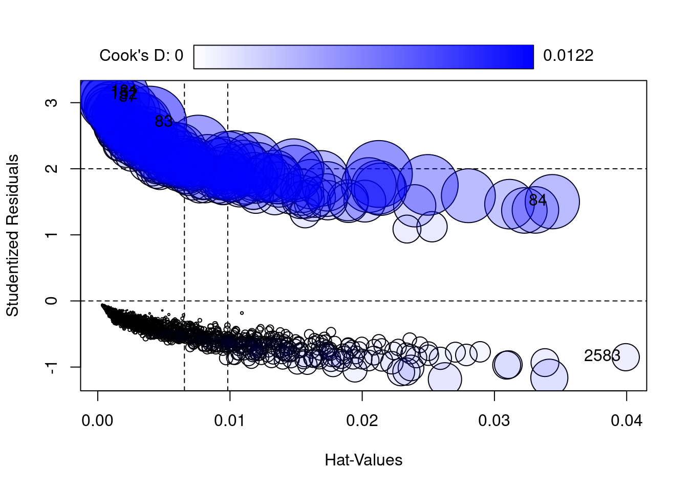
There are several assumptions for Logistic Regression: 1. The Dependent Variable is binary (i.e, 0 or 1) 2. There is a linear relationship between th logit of the outcome and each predictor 3. There are NO high leverage outliers in the predictors 4. There is No high multicollinearity (ie strong correlations) between predictors

Code

LR_stroke2 <- stroke1_clean
model2 <- glm(stroke ~ gender + age + hypertension + heart_disease + ever_married + work_type + Residence_type + avg_glucose_level + bmi + smoking_status, data=LR_stroke2, family = binomial)
summary(model2)


Call:
glm(formula = stroke ~ gender + age + hypertension + heart_disease + 
    ever_married + work_type + Residence_type + avg_glucose_level + 
    bmi + smoking_status, family = binomial, data = LR_stroke2)

Coefficients:
                   Estimate Std. Error z value Pr(>|z|)    
(Intercept)       -8.426854   0.873243  -9.650  < 2e-16 ***
gender             0.080370   0.167274   0.480 0.630893    
age                0.070967   0.006845  10.368  < 2e-16 ***
hypertension       0.570797   0.182580   3.126 0.001770 ** 
heart_disease      0.417884   0.220311   1.897 0.057856 .  
ever_married       0.174316   0.261832   0.666 0.505569    
work_type         -0.109615   0.126101  -0.869 0.384703    
Residence_type     0.005932   0.162188   0.037 0.970822    
avg_glucose_level  0.004658   0.001375   3.388 0.000704 ***
bmi                0.006275   0.012875   0.487 0.625954    
smoking_status     0.179921   0.106431   1.691 0.090932 .  
---
Signif. codes:  0 '***' 0.001 '**' 0.01 '*' 0.05 '.' 0.1 ' ' 1

(Dispersion parameter for binomial family taken to be 1)

    Null deviance: 1403.5  on 3356  degrees of freedom
Residual deviance: 1145.4  on 3346  degrees of freedom
AIC: 1167.4

Number of Fisher Scoring iterations: 7

3.1 Testing Assumption 1

Testing Assumption 1: The Dependent Variable is binary (0 or 1)

Code

unique(LR_stroke2$stroke)

[1] 1 0

3.2 Testing Assumption 2

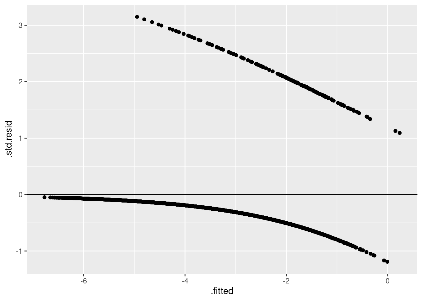
Testing Assumption 2: There is a linear relationship between the outcome variable and each predictor (use boxTidwell)

For boxTidwell, first adjust all predictors so all values are positive. If we obtain a P value greater than 0.05 it indicates a linear relationship between the predictor and the outcome.

Code

LR_stroke2$genderadj            <- LR_stroke2$gender            + abs(min(LR_stroke1$gender))            + 1
LR_stroke2$ageadj               <- LR_stroke2$age               + abs(min(LR_stroke1$age))               + 1
LR_stroke2$hypertensionadj      <- LR_stroke2$hypertension      + abs(min(LR_stroke1$hypertension))      + 1
LR_stroke2$heart_diseaseadj     <- LR_stroke2$heart_disease     + abs(min(LR_stroke1$hypertension))      + 1
LR_stroke2$ever_marriedadj      <- LR_stroke2$ever_married      + abs(min(LR_stroke1$ever_married))      + 1
LR_stroke2$work_typeadj         <- LR_stroke2$work_type         + abs(min(LR_stroke1$work_type))         + 1
LR_stroke2$Residence_typeadj    <- LR_stroke2$Residence_type    + abs(min(LR_stroke1$Residence_type))    + 1
LR_stroke2$avg_glucose_leveladj <- LR_stroke2$avg_glucose_level + abs(min(LR_stroke1$avg_glucose_level)) + 1
LR_stroke2$bmiadj               <- LR_stroke2$bmi               + abs(min(LR_stroke1$bmi))               + 1
LR_stroke2$smoking_statusadj    <- LR_stroke2$smoking_status    + abs(min(LR_stroke1$smoking_status))    + 1

Error in linearHypothesis.lm(mod.2, H) : there are aliased coefficients in the model.

Code

# boxTidwell(stroke ~ genderadj + ageadj + hypertensionadj + heart_diseaseadj + ever_marriedadj + work_typeadj + Residence_typeadj + avg_glucose_leveladj + bmiadj + smoking_statusadj, data=LR_stroke2)

3.2.1 Issues Testing Assumption 2

Trying to Drop Aliased Predictors

Code

# First, create the linear model object
lm_model <- lm(stroke ~ genderadj + ageadj + hypertensionadj + heart_diseaseadj + ever_marriedadj + work_typeadj + Residence_typeadj + avg_glucose_leveladj + bmiadj + smoking_statusadj, data=LR_stroke2)

# Then, run the alias() function
alias(lm_model)

Model :
stroke ~ genderadj + ageadj + hypertensionadj + heart_diseaseadj + 
    ever_marriedadj + work_typeadj + Residence_typeadj + avg_glucose_leveladj + 
    bmiadj + smoking_statusadj

Code

# Model : stroke ~ genderadj + ageadj + hypertensionadj + heart_diseaseadj + ever_marriedadj + work_typeadj + Residence_typeadj + avg_glucose_leveladj + bmiadj + smoking_statusadj

You can also check for perfect correlation and see if any correlations are ±1.

Code

cor(LR_stroke2[, c("genderadj","ageadj","hypertensionadj","heart_diseaseadj",
                   "ever_marriedadj","work_typeadj","Residence_typeadj",
                   "avg_glucose_leveladj","bmiadj","smoking_statusadj")])

                       genderadj      ageadj hypertensionadj heart_diseaseadj
genderadj             1.00000000 -0.05599748    -0.040011423     -0.104191111
ageadj               -0.05599748  1.00000000     0.263123514      0.260353361
hypertensionadj      -0.04001142  0.26312351     1.000000000      0.110020853
heart_diseaseadj     -0.10419111  0.26035336     0.110020853      1.000000000
ever_marriedadj       0.02728003 -0.48775310    -0.107114849     -0.069804764
work_typeadj          0.01495643  0.14214267     0.048358096      0.029618537
Residence_typeadj    -0.01143732 -0.01761422     0.003112702     -0.010250014
avg_glucose_leveladj -0.07148597  0.23864619     0.168909926      0.143333385
bmiadj               -0.01991382  0.04222590     0.127363138     -0.003962827
smoking_statusadj    -0.07723370  0.03463196    -0.005416806      0.060198195
                     ever_marriedadj work_typeadj Residence_typeadj
genderadj                 0.02728003  0.014956427      -0.011437323
ageadj                   -0.48775310  0.142142673      -0.017614219
hypertensionadj          -0.10711485  0.048358096       0.003112702
heart_diseaseadj         -0.06980476  0.029618537      -0.010250014
ever_marriedadj           1.00000000 -0.020663455       0.011239966
work_typeadj             -0.02066345  1.000000000      -0.007197831
Residence_typeadj         0.01123997 -0.007197831       1.000000000
avg_glucose_leveladj     -0.11858810  0.034327248       0.008010375
bmiadj                   -0.12527547 -0.017017707       0.009836168
smoking_statusadj        -0.05723324 -0.015271022      -0.039896247
                     avg_glucose_leveladj       bmiadj smoking_statusadj
genderadj                    -0.071485971 -0.019913816      -0.077233702
ageadj                        0.238646187  0.042225902       0.034631959
hypertensionadj               0.168909926  0.127363138      -0.005416806
heart_diseaseadj              0.143333385 -0.003962827       0.060198195
ever_marriedadj              -0.118588103 -0.125275472      -0.057233241
work_typeadj                  0.034327248 -0.017017707      -0.015271022
Residence_typeadj             0.008010375  0.009836168      -0.039896247
avg_glucose_leveladj          1.000000000  0.155139559       0.005095349
bmiadj                        0.155139559  1.000000000       0.029041449
smoking_statusadj             0.005095349  0.029041449       1.000000000

check constant columns:

If any variable only has one unique value → it’s constant → alias.

Code

sapply(LR_stroke2, function(x) length(unique(x)))

              gender                  age         hypertension 
                   2                   70                    2 
       heart_disease         ever_married            work_type 
                   2                    2                    4 
      Residence_type    avg_glucose_level                  bmi 
                   2                 2861                  364 
      smoking_status               stroke            genderadj 
                   3                    2                    2 
              ageadj      hypertensionadj     heart_diseaseadj 
                  70                    2                    2 
     ever_marriedadj         work_typeadj    Residence_typeadj 
                   2                    4                    2 
avg_glucose_leveladj               bmiadj    smoking_statusadj 
                2861                  364                    3

Error in linearHypothesis.lm(mod.2, H) : there are aliased coefficients in the model.

Code

# boxTidwell(stroke ~ genderadj + ageadj + hypertensionadj + heart_diseaseadj + ever_marriedadj + work_typeadj + Residence_typeadj + avg_glucose_leveladj + bmiadj + smoking_statusadj, data=LR_stroke2)

3.3 Testing Assumption 3

Testing Assumption 3: assess influential outliers using car package and influencePlot

Code

car::influencePlot(model2)

        StudRes          Hat       CookD
83    2.6917353 0.0039267816 0.012237368
84    1.5018344 0.0343771041 0.006641860
87    3.0732709 0.0012042796 0.011476828
131   3.1608870 0.0006013465 0.007697762
152   3.1135601 0.0005613972 0.006237531
2583 -0.8509399 0.0399302730 0.001668526

3.4 Testing Assumption 4

Testing Assumption 4 : Multicollinearity using ggplot and augment

Code

# Testing Assumption 4 : Multicollinearity using ggplot and augment#
aug <- augment(model2)
ggplot(aug,aes(.fitted, .std.resid)) + geom_point() + geom_hline(yintercept=0)

3.5 Conclusion of Testing Assumptions

Conclusion: Now that all 4 assumptions are met, logistic regression is a valid model to analyze the model

4 Analysis of the Model

Part 4: Analysis of the Model

Code

model2 <- glm(stroke ~ gender + age + hypertension + heart_disease + ever_married + work_type + Residence_type + avg_glucose_level + bmi + smoking_status, data=LR_stroke2, family = binomial)
summary(model2)


Call:
glm(formula = stroke ~ gender + age + hypertension + heart_disease + 
    ever_married + work_type + Residence_type + avg_glucose_level + 
    bmi + smoking_status, family = binomial, data = LR_stroke2)

Coefficients:
                   Estimate Std. Error z value Pr(>|z|)    
(Intercept)       -8.426854   0.873243  -9.650  < 2e-16 ***
gender             0.080370   0.167274   0.480 0.630893    
age                0.070967   0.006845  10.368  < 2e-16 ***
hypertension       0.570797   0.182580   3.126 0.001770 ** 
heart_disease      0.417884   0.220311   1.897 0.057856 .  
ever_married       0.174316   0.261832   0.666 0.505569    
work_type         -0.109615   0.126101  -0.869 0.384703    
Residence_type     0.005932   0.162188   0.037 0.970822    
avg_glucose_level  0.004658   0.001375   3.388 0.000704 ***
bmi                0.006275   0.012875   0.487 0.625954    
smoking_status     0.179921   0.106431   1.691 0.090932 .  
---
Signif. codes:  0 '***' 0.001 '**' 0.01 '*' 0.05 '.' 0.1 ' ' 1

(Dispersion parameter for binomial family taken to be 1)

    Null deviance: 1403.5  on 3356  degrees of freedom
Residual deviance: 1145.4  on 3346  degrees of freedom
AIC: 1167.4

Number of Fisher Scoring iterations: 7

Conclusion: age, hypertension, heartdisease, and avg_glucose_level are statistically significant predictors on whether one has a stroke or not.

all the P values of these 4 predictors is .05 or less (note included heart_disease because it approaches statistical significance at .057)

Since this a logistic regression, we cant use R squared and adjusted R squared to see how well the model predicted stroke. So we substitute McFadden’s P value.

Code

# install.packages("pscl")
# library(pscl)
pR2(model2)

fitting null model for pseudo-r2

          llh       llhNull            G2      McFadden          r2ML 
-572.70320797 -701.73792863  258.06944131    0.18387879    0.07399442 
         r2CU 
   0.21655630

Comment McFadden = .18– not a bad fit for logistic regression

Create a confusion matrix (Type1 vs Type2 error in statistics)

Code

# install.packages("parallelly")
# install.packages("cli")
# library(caret)

# Predict probabilities from the logistic regression model
predicted_prob1 <- predict(model2, type = "response")

# Convert probabilities to binary classes using a 0.5 cutoff
predicted_class1 <- ifelse(predicted_prob1 > 0.5, 1, 0)

predicted_class1 <- factor(predicted_class1, levels = c(0,1))
ForReal_Stroke1 <- factor(LR_stroke2$stroke, levels = c(0,1))
confusionMatrix(predicted_class1, ForReal_Stroke1)

Confusion Matrix and Statistics

          Reference
Prediction    0    1
         0 3177  178
         1    0    2
                                          
               Accuracy : 0.947           
                 95% CI : (0.9388, 0.9543)
    No Information Rate : 0.9464          
    P-Value [Acc > NIR] : 0.4587          
                                          
                  Kappa : 0.0208          
                                          
 Mcnemar's Test P-Value : <2e-16          
                                          
            Sensitivity : 1.00000         
            Specificity : 0.01111         
         Pos Pred Value : 0.94694         
         Neg Pred Value : 1.00000         
             Prevalence : 0.94638         
         Detection Rate : 0.94638         
   Detection Prevalence : 0.99940         
      Balanced Accuracy : 0.50556         
                                          
       'Positive' Class : 0

Analysis of the Confusion Matrix: Crud…poor results

Further Analysis of the Confusion Matrix with F1 score and Precision Recall

4.1 F1 Score and Precision Recall

Precision - out of all the true strokes the model predicted, how many really were strokes? = 1 = 100%

Code

precision1 <- sum((predicted_class1 == 1) & (ForReal_Stroke1 == 1)) / sum(predicted_class1 == 1)

Recall - out of all the actual strokes, how many did the model catch?

Results = .01 or 1%—

Code

recall1 <- sum((predicted_class1 == 1) & (ForReal_Stroke1 == 1)) / sum(ForReal_Stroke1 == 1)

f1_Score - How well does this model predict strokes?

Results = .022 or 2.2% –very poorly

Code

f1_score1  <- 2 * precision1 * recall1 / (precision1 + recall1)

precision1, recall1, f1_score1

Code

precision1

[1] 1

Code

recall1

[1] 0.01111111

Code

f1_score1

[1] 0.02197802

Conclusion

Ideas for improving precision, recall and f1_score
Address imbalance by upsample (add stroke cases), downsample (remove non strokecases) and or SMOTE (Synthetic data)
Change the classification threshold
Compare with Alternative Models such as random forrests or XGBoost

References

1. fedesoriano. (n.d.). Stroke Prediction Dataset. https://www.kaggle.com/datasets/fedesoriano/stroke-prediction-dataset