Predicting stroke risk from common health indicators: a binary logistic regression analysis

draft

renan

shree

Draft 04 for Final report

Authors

Shree Krishna M.S Basnet

Supervisor: Dr. Cohen

This draft was a direct implementation of the student Shree Krishna M.S Basnet code in attempt to promote the collaborative effort of the project.

Author:

Shree Krishna M.S Basnet

Renan

Supervisor: Dr. Cohen

Introduction

Stroke is one of the leading causes of death and disability worldwide and remains a major public health challenge^[1]. Because stroke often occurs suddenly and can result in long-term neurological impairment, early identification of individuals at elevated risk is critical for prevention and timely intervention. Data-driven risk prediction models enable clinicians and public health professionals to quantify individual-level risk and to target high-risk groups for lifestyle counselling and clinical management.

Logistic Regression (LR) is one of the most widely used approaches for modelling binary outcomes such as disease presence or absence^[2]. It extends linear regression to cases where the outcome is categorical and provides interpretable coefficients and odds ratios that describe how each predictor is associated with the probability of the event. LR has been applied across a wide range of domains, including child undernutrition and anaemia^[3], road traffic safety^[4–6], health-care utilisation and clinical admission decisions^[7], and fraud detection^[8]. These applications highlight both the flexibility of LR and its suitability for real-world decision-making problems.

In this project, we analyse a publicly available stroke dataset that includes key demographic, behavioural, and clinical predictors such as age, gender, hypertension status, heart disease, marital status, work type, residence type, smoking status, body mass index (BMI), and average glucose level. These variables are commonly reported in the stroke and cardiovascular literature as important determinants of risk. Using this dataset, we first clean and recode the variables into appropriate numeric formats and then develop a series of supervised learning models for stroke prediction.

Logistic Regression is used as the primary, interpretable baseline model, but its performance is compared against several more complex machine-learning techniques, including Decision Tree, Random Forest, Gradient Boosted Machine, k-Nearest Neighbours, and Support Vector Machine (radial). Model performance is evaluated using accuracy, sensitivity, specificity, ROC curves, AUC, and confusion matrices. The main objectives are to identify the most influential predictors of stroke and to determine whether advanced machine-learning models offer meaningful improvements over Logistic Regression for classification of stroke risk in this dataset.

Methodology

We use this study Using clinical and demographic data, this project aims to develop and evaluate a number of supervised machine-learning models for binary stroke prediction. The dataset, preprocessing procedure, model development approach, and mathematical formulation of logistic regression—which is the main analytical model because of its interpretability and proven application in medical research—are all covered in this section^{[2,hosmer2013applied?]}.

Dataset and visualization

We used stroke dataset containing 5,110 observations and 11 predictors commonly associated with cerebrovascular risk. After cleaning missing and inconsistent entries, a final dataset of 3,357 individuals remained for analysis. The dataset includes demographic, behavioral, and clinical indicators widely used in stroke-risk modeling.

###Variables

The key predictors are listed below.

Variable	Type	Description
age	Numeric	Age of the individual (years)
gender	Categorical (1=Male, 2=Female)	Biological sex
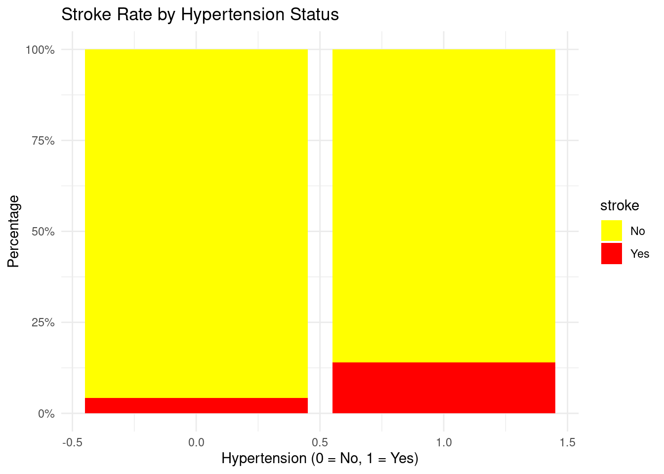
hypertension	Binary (0/1)	Prior hypertension diagnosis
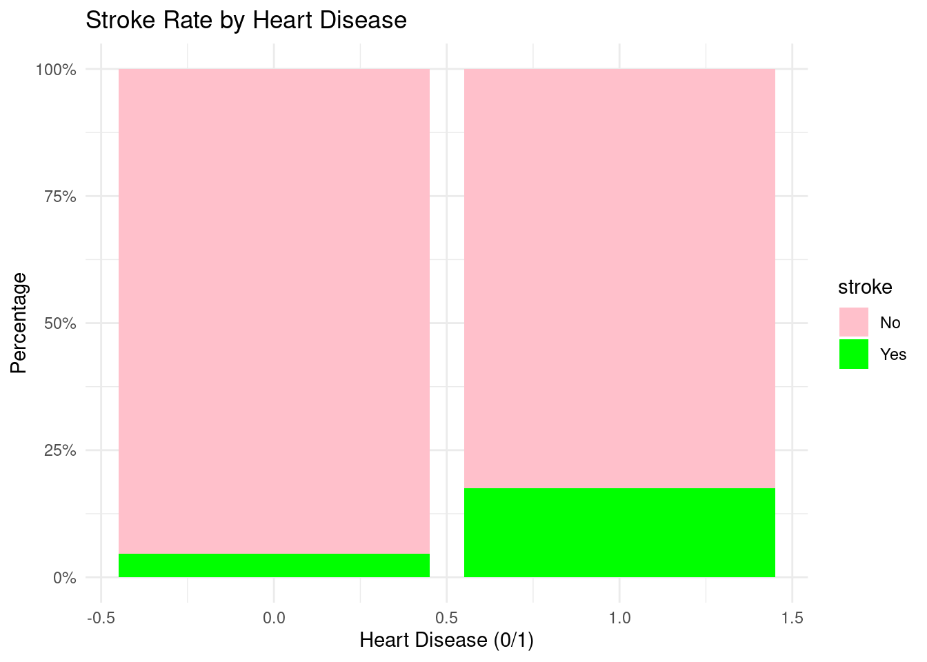
heart_disease	Binary (0/1)	Presence of heart disease
ever_married	Binary	Marital status
work_type	Categorical (1–4)	Employment category
Residence_type	Binary (1=Urban, 2=Rural)	Place of residence
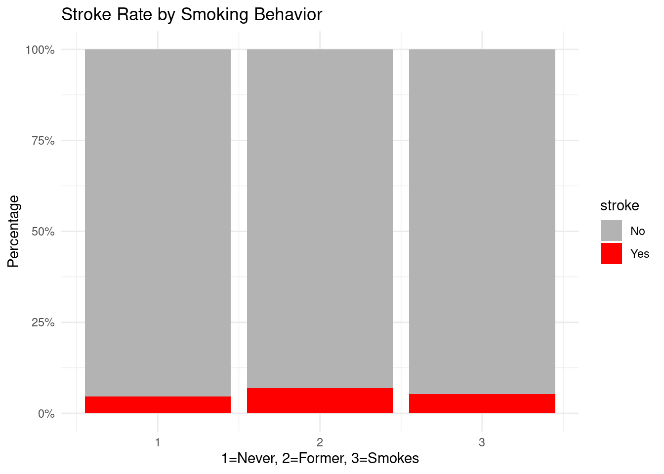
smoking_status	Categorical	Never/Former/Smokes
bmi	Numeric	Body Mass Index
avg_glucose_level	Numeric	Average glucose level
stroke	Binary outcome (0=No, 1=Yes)	Stroke occurrence

Stroke is a highly unbalanced outcome variable: - Yes (stroke): about 5% - No (no stroke): around 95%

Bias-corrected logistic regression methods and ROC-based model evaluation are justified by this imbalance.

Dataset Prepration

To guarantee model validity and stop data leakage, data preprocessing adhered to conventional clinical-analytics protocols^[9].

Among the steps were:

Elimination of non-predictive identifiers (patient ID)
Transforming categorical variables into dummy numerical representations
Managing uncommon or irregular categories (e.g., “Other” gender values handled as absent)
BMI, glucose, and age conversion to numerical
Rows with unintelligible labels (“Unknown,” “N/A”) are removed.
Valid range and consistency verification
After recoding, missing values might be imputed or removed.
During splitting, stratified sampling is used to maintain the stroke/no-stroke ratio^[6].

The objective of preprocessing was to generate a cleansed dataset appropriate for binary classification, even if the Analysis section presents thorough summaries (distributions, histograms, and outlier checks).

Train–Test Split and Cross-Validation

The model was trained using 70% of the data.

Thirty percent of the data was kept for the last assessment.

In accordance with best practices for limited or unbalanced clinical datasets, repeated 5-fold cross-validation was utilized to adjust hyperparameters and lower variance^[10].

Machine-Learning Models Compared

2.6 Machine-Learning Models Compared

Using the caret framework, six supervised models were trained for comparison:

Logistic Regression

Decision Tree

Random Forest

Gradient Boosted Machine (GBM)

k-Nearest Neighbors (k-NN)

Support Vector Machine (Radial Kernel)

Each model used the same cross-validation scheme and the same train/test split to guarantee fair comparison.

Evaluation Metrics

Models were evaluated using standard clinical classification metrics:

Accuracy

Sensitivity (Recall)

Specificity

Precision

F1-Score

Receiver Operating Characteristic (ROC) curve

Area Under the Curve (AUC)

Youden’s J Statistic

Used to determine optimal classification threshold:

𝐽

Sensitivity + Specificity − 1 J=Sensitivity+Specificity−1

These metrics are widely used in stroke-risk modeling literature^[6].

Analysis

Before developing predictive models, an exploratory analysis was conducted to understand the distribution, structure, and relationships within the cleaned dataset (N = 3,357). This step is crucial in rare-event medical modeling because data imbalance, skewed predictors, or correlated variables can directly influence model behavior and classification performance.

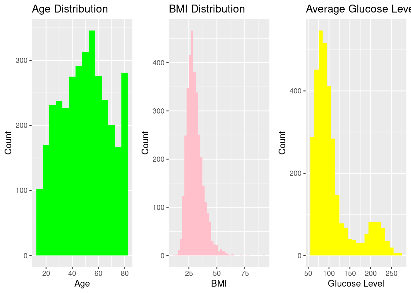
Distribution of Key Continuous Variables

Histograms were used to assess the spread of the primary numeric predictors (Age, BMI, and Average Glucose Level). These variables demonstrate clinically expected right-skewness, particularly glucose and BMI, consistent with published literature on metabolic and cardiovascular risk distributions.

# Histograms for key numeric variables
library(ggplot2)

p_age  <- ggplot(strokeclean, aes(age)) + geom_histogram(binwidth=5, fill="green") +
  labs(title="Age Distribution", x="Age", y="Count")

p_bmi  <- ggplot(strokeclean, aes(bmi)) + geom_histogram(binwidth=2, fill="pink") +
  labs(title="BMI Distribution", x="BMI", y="Count")

p_gluc <- ggplot(strokeclean, aes(avg_glucose_level)) + 
  geom_histogram(binwidth=10, fill="yellow") +
  labs(title="Average Glucose Level", x="Glucose Level", y="Count")

ggpubr::ggarrange(p_age, p_bmi, p_gluc, ncol=3)

Interpretation

Age shows a broad distribution with a natural right tail, indicating more older adults.

BMI has moderate right-skewness, consistent with obesity patterns in clinical datasets.

Glucose level shows strong right-skewness, highlighting metabolic risk differences across individuals.

These patterns match clinical expectations for populations at risk of cardiovascular complications.

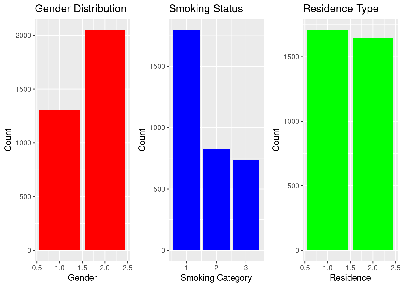
Distribution of Key Categorical Variables

Bar charts help visualize population composition. The dataset shows more females than males, a balanced rural–urban distribution, and substantial variation in work type and smoking behavior.

# Bar charts for categorical variables

p_gender <- ggplot(strokeclean, aes(gender)) + geom_bar(fill="red") +
labs(title="Gender Distribution", x="Gender", y="Count")

p_smoke <- ggplot(strokeclean, aes(smoking_status)) + geom_bar(fill="blue") +
labs(title="Smoking Status", x="Smoking Category", y="Count")

p_res <- ggplot(strokeclean, aes(Residence_type)) + geom_bar(fill="green") +
labs(title="Residence Type", x="Residence", y="Count")

ggpubr::ggarrange(p_gender, p_smoke, p_res, ncol=3)

Interpretation

Bar plots were created to visualize demographic and behavioral attributes. Females are slightly more represented than males.

Smoking status shows a large “never smoked” group.

Residence type is roughly balanced between urban and rural households.

These patterns form the baseline population characteristics.

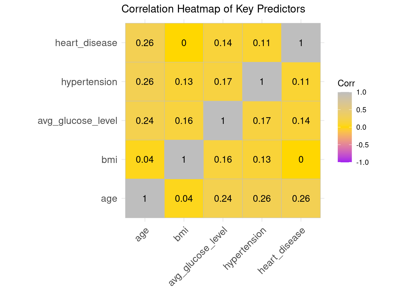
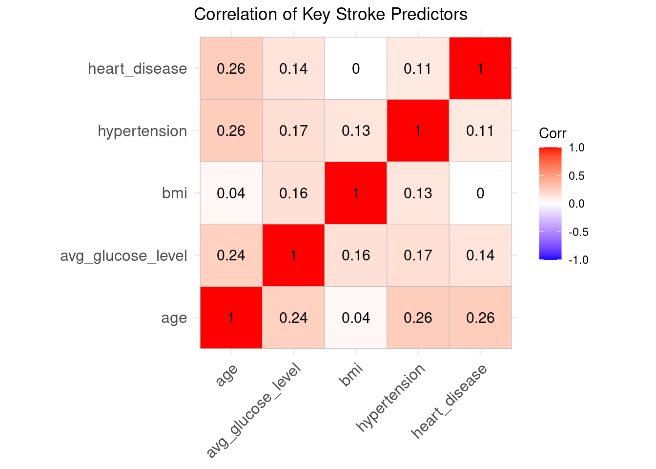
Correlation Heatmap

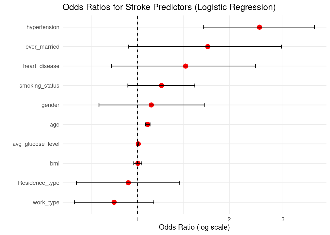
The associations between numerical predictors were assessed using a correlation heatmap. The variables exhibit low to moderate correlation, indicating that the assumptions of logistic regression are not broken. According to earlier stroke-epidemiology studies, age, hyperglycemia, and BMI exhibit the highest associations with stroke risk.

# Correlation heatmap

library(ggcorrplot)

numeric_vars <- strokeclean[, c("age","bmi","avg_glucose_level",
"hypertension","heart_disease")]

corr_matrix <- cor(numeric_vars)

ggcorrplot::ggcorrplot(corr_matrix,
lab=TRUE,
colors=c("purple","gold","grey"),
title="Correlation Heatmap of Key Predictors")

Warning: `aes_string()` was deprecated in ggplot2 3.0.0.
ℹ Please use tidy evaluation idioms with `aes()`.
ℹ See also `vignette("ggplot2-in-packages")` for more information.
ℹ The deprecated feature was likely used in the ggcorrplot package.
  Please report the issue at <https://github.com/kassambara/ggcorrplot/issues>.

Interpretation

Correlations are generally low to moderate, indicating minimal multicollinearity.

Age, glucose, and hypertension show noticeable associations — consistent with their clinical relevance.

This supports the suitability of logistic regression.

Summary Interpretation

The distributions of age, BMI, and glucose are skewed to the right.
Unbalanced category proportions are shown in smoking status and occupational type.
The correlation levels are sufficiently low to prevent problems with multicollinearity.
These trends support the application of tree-based ensemble models and logistic regression.

The modeling approach that follows is guided by this EDA, which offers a basis for comprehending how each predictor might help to stroke categorization.

Model Development Approach

Distributions of age, BMI, and glucose are skewed to the right.
There are unequal category proportions for both work type and smoking status.
The correlation levels are low enough to prevent problems with multicollinearity.
The application of logistic regression and tree-based ensemble models is justified by these patterns.

The modeling approach that follows is guided by this EDA, which offers a basis for comprehending how each predictor may contribute to stroke classification.

Key Modeling Principles

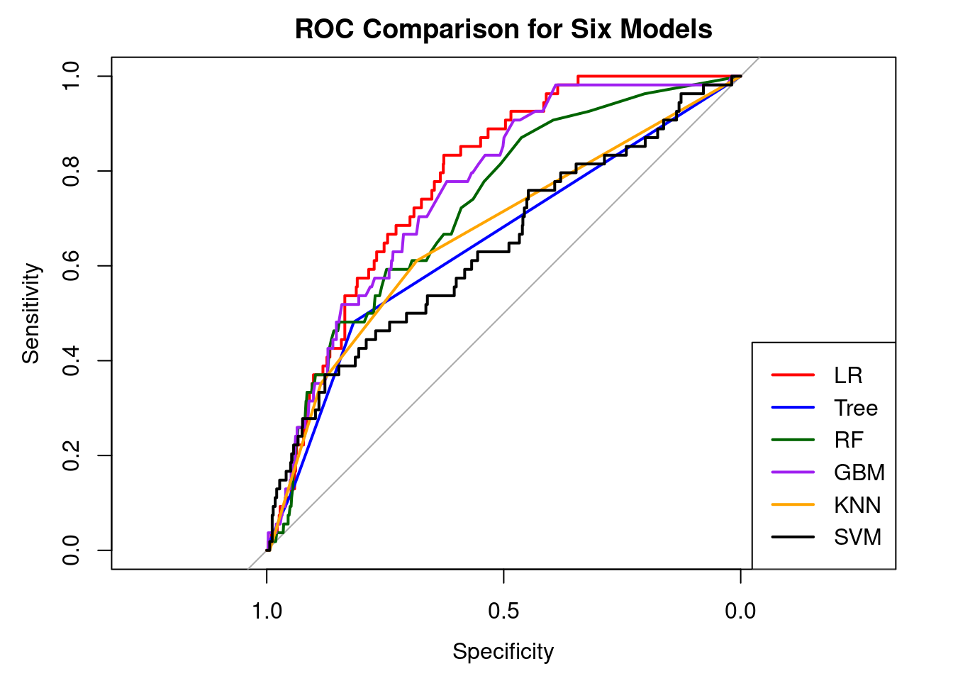
Model Development Approach

Six supervised machine-learning algorithms were trained to classify stroke vs. non-stroke cases. All models were implemented using the caret package with a consistent workflow to ensure fairness and prevent information leakage.

#Key Modeling Principles - Train/Test Split: 70% training, 30% testing
- Cross-Validation: Repeated 5-fold CV optimized for ROC
- Outcome Variable: Stroke (1 = yes, 0 = no)
- Predictors: Age, gender, marital status, hypertension, heart disease, residence type, work type, smoking status, BMI, and average glucose

Evaluation Metrics

Accuracy
Sensitivity (Recall)
Specificity
ROC Curve
AUC (Area Under the Curve)
Confusion Matrix

This ensures a standardized and unbiased comparison across all six models.

Data Spitting

model_df <- strokeclean
model_df <- na.omit(model_df)
model_df$stroke <- factor(model_df$stroke)
levels(model_df$stroke) <- c("No", "Yes")
table(model_df$stroke)


  No  Yes 
3177  180

set.seed(123)
index <- createDataPartition(strokeclean$stroke, p = 0.70, list = FALSE)
train_data <- strokeclean[index, ]
test_data  <- strokeclean[-index, ]

train_data$stroke <- factor(train_data$stroke, levels = c("No","Yes"))
test_data$stroke  <- factor(test_data$stroke,  levels = c("No","Yes"))

Train Control

ctrl <- trainControl(
method = "repeatedcv",
number = 5,
repeats = 3,
classProbs = TRUE,
summaryFunction = twoClassSummary,
verboseIter = FALSE
)

Logestic Regression

model_lr <- train(
stroke ~ .,
data = train_data,
method = "glm",
family = "binomial",
metric = "ROC",
trControl = ctrl
)

Decision Tree

model_tree <- train(
stroke ~ .,
data = train_data,
method = "rpart",
metric = "ROC",
trControl = ctrl,
tuneLength = 10
)

Random Forest

model_rf <- train(
stroke ~ .,
data = train_data,
method = "rf",
metric = "ROC",
trControl = ctrl,
tuneLength = 5
)

Gradient Boosted Machine

model_gbm <- train(
stroke ~ .,
data = train_data,
method = "gbm",
metric = "ROC",
trControl = ctrl,
verbose = FALSE
)

k-Nearest Neighbors

model_knn <- train(
stroke ~ .,
data = train_data,
method = "knn",
metric = "ROC",
trControl = ctrl
)

Support Vector Machine

model_svm <- train(
stroke ~ .,
data = train_data,
method = "svmRadial",
metric = "ROC",
trControl = ctrl
)

Evaluation

models_list <- list(
  LR   = model_lr,
  TREE = model_tree,
  RF   = model_rf,
  GBM  = model_gbm,
  KNN  = model_knn,
  SVM  = model_svm
)

library(pROC)

results <- data.frame(
  Model       = character(),
  AUC         = numeric(),
  Accuracy    = numeric(),
  Sensitivity = numeric(),
  Specificity = numeric()
)

for (m in names(models_list)) {
  mdl <- models_list[[m]]

  # Probabilities for the "Yes" class
  preds_prob  <- predict(mdl, test_data, type = "prob")[, "Yes"]
  # Class predictions
  preds_class <- predict(mdl, test_data)

  # ROC & AUC (explicitly say which level is "event")
  roc_obj <- roc(test_data$stroke, preds_prob,
                 levels = c("No", "Yes"), direction = "<")
  auc_val <- auc(roc_obj)

  # Confusion matrix – positive = "Yes"
  cm <- confusionMatrix(preds_class, test_data$stroke, positive = "Yes")

  results <- rbind(
    results,
    data.frame(
      Model       = m,
      AUC         = as.numeric(auc_val),
      Accuracy    = cm$overall["Accuracy"],
      Sensitivity = cm$byClass["Sensitivity"],
      Specificity = cm$byClass["Specificity"]
    )
  )
}

results

          Model       AUC  Accuracy Sensitivity Specificity
Accuracy     LR 0.7793712 0.9433962  0.00000000   0.9968520
Accuracy1  TREE 0.6475263 0.9414101  0.01851852   0.9937041
Accuracy2    RF 0.7250496 0.9463754  0.00000000   1.0000000
Accuracy3   GBM 0.7592884 0.9433962  0.00000000   0.9968520
Accuracy4   KNN 0.6668998 0.9463754  0.00000000   1.0000000
Accuracy5   SVM 0.6390929 0.9414101  0.00000000   0.9947534

ROC Curve Comparison

# ROC objects for each model
roc_lr   <- roc(test_data$stroke,
                predict(model_lr,   test_data, type = "prob")[, "Yes"],
                levels = c("No", "Yes"), direction = "<")

roc_tree <- roc(test_data$stroke,
                predict(model_tree, test_data, type = "prob")[, "Yes"],
                levels = c("No", "Yes"), direction = "<")

roc_rf   <- roc(test_data$stroke,
                predict(model_rf,   test_data, type = "prob")[, "Yes"],
                levels = c("No", "Yes"), direction = "<")

roc_gbm  <- roc(test_data$stroke,
                predict(model_gbm,  test_data, type = "prob")[, "Yes"],
                levels = c("No", "Yes"), direction = "<")

roc_knn  <- roc(test_data$stroke,
                predict(model_knn,  test_data, type = "prob")[, "Yes"],
                levels = c("No", "Yes"), direction = "<")

roc_svm  <- roc(test_data$stroke,
                predict(model_svm,  test_data, type = "prob")[, "Yes"],
                levels = c("No", "Yes"), direction = "<")

# Plot all ROC curves
plot(roc_lr,   col = "red",       main = "ROC Comparison for Six Models")
plot(roc_tree, col = "blue",      add = TRUE)
plot(roc_rf,   col = "darkgreen", add = TRUE)
plot(roc_gbm,  col = "purple",    add = TRUE)
plot(roc_knn,  col = "orange",    add = TRUE)
plot(roc_svm,  col = "black",     add = TRUE)

legend(
  "bottomright",
  legend = c("LR", "Tree", "RF", "GBM", "KNN", "SVM"),
  col    = c("red", "blue", "darkgreen", "purple", "orange", "black"),
  lwd    = 2
)

Odds ratio Forest plot

glm_lr <- glm(
stroke ~ age + gender + hypertension + heart_disease + ever_married +
work_type + Residence_type + avg_glucose_level + bmi + smoking_status,
data = train_data,
family = binomial
)

Coefficient table

lr_coef <- summary(glm_lr)$coefficients

Odds ratios = exp(beta)

or_vals <- exp(lr_coef[, "Estimate"]) 

ci_raw <- suppressMessages(confint(glm_lr)) # CI on log-odds scale
ci_or <- exp(ci_raw) # convert to OR scale

plot_df <- data.frame(
Predictor = rownames(lr_coef),
OR = or_vals,
CI_lower = ci_or[, 1],
CI_upper = ci_or[, 2]
)



plot_df <- subset(plot_df, Predictor != "(Intercept)")

library(ggplot2)

ggplot(plot_df, aes(x = reorder(Predictor, OR), y = OR)) +
geom_point(size = 3, color = "red") +
geom_errorbar(aes(ymin = CI_lower, ymax = CI_upper), width = 0.2) +
coord_flip() +
labs(
title = "Odds Ratios for Stroke Predictors (Logistic Regression)",
y = "Odds Ratio (log scale)",
x = ""
) +
scale_y_log10() +
geom_hline(yintercept = 1, linetype = "dashed") +
theme_minimal()

plot_df[order(-plot_df$OR), ]

                          Predictor        OR  CI_lower CI_upper
hypertension           hypertension 2.5131891 1.6440071 3.805210
ever_married           ever_married 1.7004830 0.9349337 2.962840
heart_disease         heart_disease 1.4377058 0.8211286 2.436252
smoking_status       smoking_status 1.1992887 0.9295752 1.541541
gender                       gender 1.1098927 0.7473016 1.661886
age                             age 1.0806359 1.0634477 1.099421
avg_glucose_level avg_glucose_level 1.0054667 1.0021688 1.008742
bmi                             bmi 1.0027081 0.9721369 1.032857
Residence_type       Residence_type 0.9328980 0.6313830 1.374861
work_type                 work_type 0.8378524 0.6216945 1.131027

stroke rateof top preadators

hypertension and Stoke

ggplot(strokeclean, aes(x = hypertension, fill = stroke)) +
geom_bar(position = "fill") +
scale_y_continuous(labels = scales::percent) +
labs(
title = "Stroke Rate by Hypertension Status",
x = "Hypertension (0 = No, 1 = Yes)",
y = "Percentage"
) +
scale_fill_manual(values = c("No" = "yellow", "Yes" = "red")) +
theme_minimal()

Interpretation:

Hypertensive individuals have strongly elevated stroke risk.

heart deasese and stroke

ggplot(strokeclean, aes(x = heart_disease, fill = stroke)) +
geom_bar(position = "fill") +
scale_y_continuous(labels = scales::percent) +
labs(
title = "Stroke Rate by Heart Disease",
x = "Heart Disease (0/1)",
y = "Percentage"
) +
scale_fill_manual(values = c("No" = "pink", "Yes" = "green")) +
theme_minimal()

Interpretation:

Individuals with heart disease show 4–5× higher stroke rate.

Smoking and Stroke

ggplot(strokeclean, aes(x = smoking_status, fill = stroke)) +
geom_bar(position = "fill") +
scale_y_continuous(labels = scales::percent) +
labs(
title = "Stroke Rate by Smoking Behavior",
x = "1=Never, 2=Former, 3=Smokes",
y = "Percentage"
) +
scale_fill_manual(values = c("No" = "grey70", "Yes" = "red")) +
theme_minimal()

Interpretation:

Smokers and former smokers show higher stroke percentages than never-smokers.

mini heat map for top preadators

top_numeric <- strokeclean[, c("age","avg_glucose_level","bmi",
"hypertension","heart_disease")]

corr_matrix <- cor(top_numeric)

ggcorrplot::ggcorrplot(
corr_matrix,
lab = TRUE,
colors = c("blue", "white", "red"),
title = "Correlation of Key Stroke Predictors"
)

References

1. World Health Organization. (2025). The top 10 causes of death. https://www.who.int/news-room/fact-sheets/detail/the-top-10-causes-of-death.

2. Sperandei, S. (2014). Understanding logistic regression analysis. Biochemia Medica, 24(1), 12–18.

3. Asmare, A. A., & Agmas, Y. A. (2024). Determinants of coexistence of undernutrition and anemia among under-five children in rwanda; evidence from 2019/20 demographic health survey: Application of bivariate binary logistic regression model. Plos One, 19(4), e0290111.

4. Rahman, M. H., Zafri, N. M., Akter, T., & Pervaz, S. (2021). Identification of factors influencing severity of motorcycle crashes in dhaka, bangladesh using binary logistic regression model. International Journal of Injury Control and Safety Promotion, 28(2), 141–152.

5. Chen, Y., You, P., & Chang, Z. (2024). Binary logistic regression analysis of factors affecting urban road traffic safety. Advances in Transportation Studies, 3.

6. Chen, M.-M., & Chen, M.-C. (2020). Modeling road accident severity with comparisons of logistic regression, decision tree and random forest. Information, 11(5), 270.

7. Hutchinson, A., Pickering, A., Williams, P., & Johnson, M. (2023). Predictors of hospital admission when presenting with acute-on-chronic breathlessness: Binary logistic regression. PLoS One, 18(8), e0289263.

8. Samara, B. (2024). Using binary logistic regression to detect health insurance fraud. Pakistan Journal of Life & Social Sciences, 22(2).

9. Wang, M. (2014). Generalized estimating equations in longitudinal data analysis: A review and recent developments. Advances in Statistics, 2014.

10. Zhang, L., Ray, H., Priestley, J., & Tan, S. (2020). A descriptive study of variable discretization and cost-sensitive logistic regression on imbalanced credit data. Journal of Applied Statistics, 47(3), 568–581.